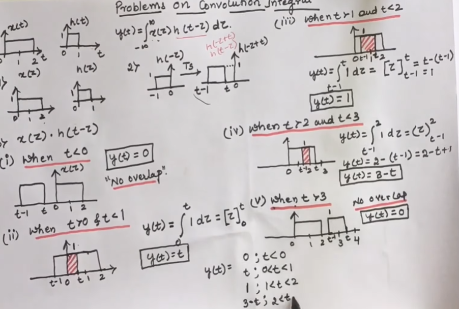
Physical quantity that contains information. Signals are expressed mathematically as function of independent variable, which is usually time.
Example:
Basic Types of Signals:
Based on Continuous and Discrete:
Continuous in Time Signal & Continuous in Value Signal
A continuous-time signal has values for all points in time in some interval.
A continuous-value signal is all possible value within an interval will be available in a signal.
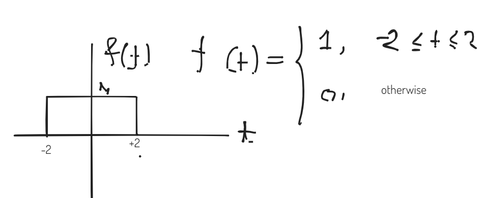
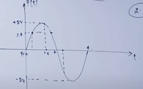
Has values for 0≤t≤4 and all values are available in the signal with -5≤v≤+5
Continuous in time but discrete in value signal
A continuous-time signal has values for all points in time in some interval.
All values within a range is not available in the signal.
Have value for time within 0≤t≤4 but all values within -5≤v≤5 is not available
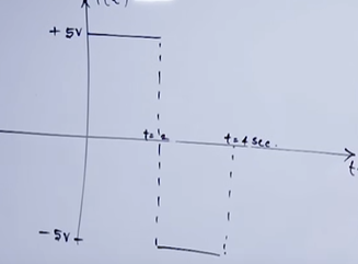
Continuous in value but discrete in time signal
Haven’t values for all points in time within an interval
All values within an range are available in a signalAll values are available, but some points in time haven’t values
Discrete in time and discrete in value signal
Analog Signal: Continuity in any of the domain (time or value)
Digital Signal: Discrete in both time and value
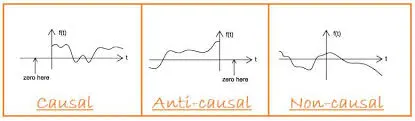
Based on Causal, Anti-Causal, Non-Causal
Causal Signals:
0 for all negative value/time
x(t)={x(t)>00t≥0t<0
Non-Causal Signals
A signal that have positive amplitude for both positive and negative instance of time
Anti-Causal Signal
0 for all positive value/time
x(t)={x(t)>00t≤0t>0
Causal, Anti-Causal, Non-Causal
Operations on Signals
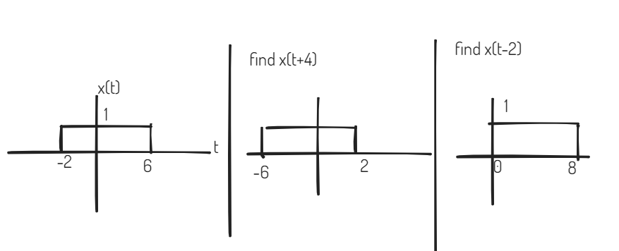
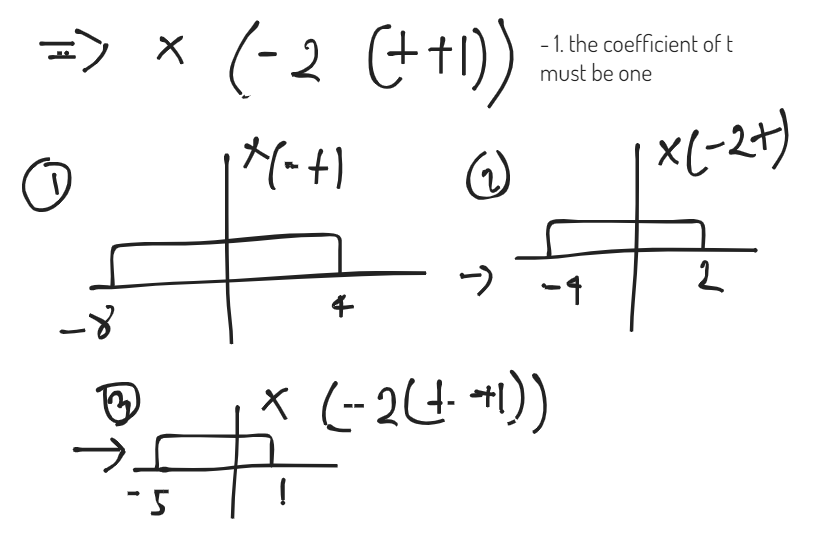
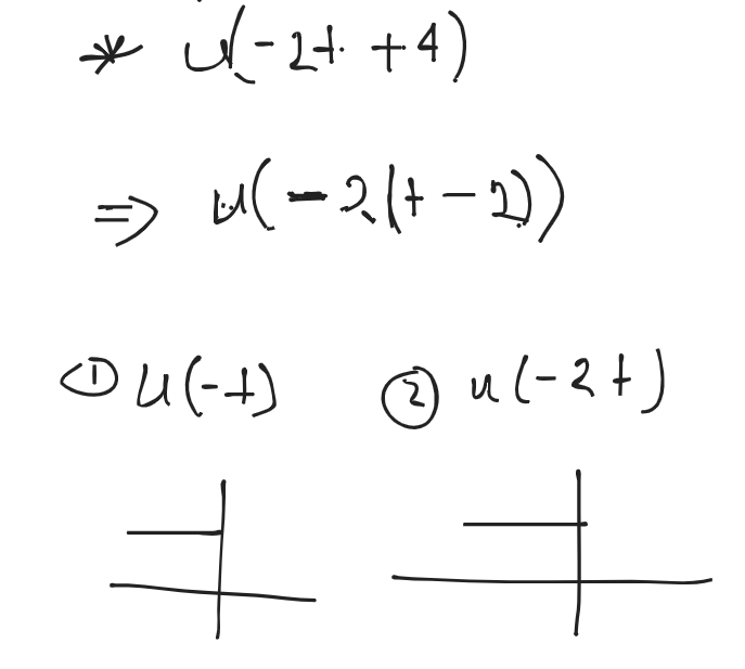
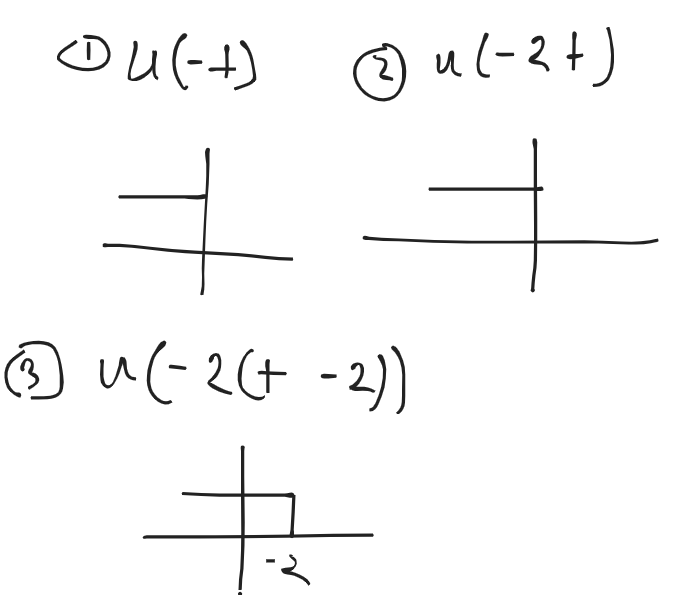
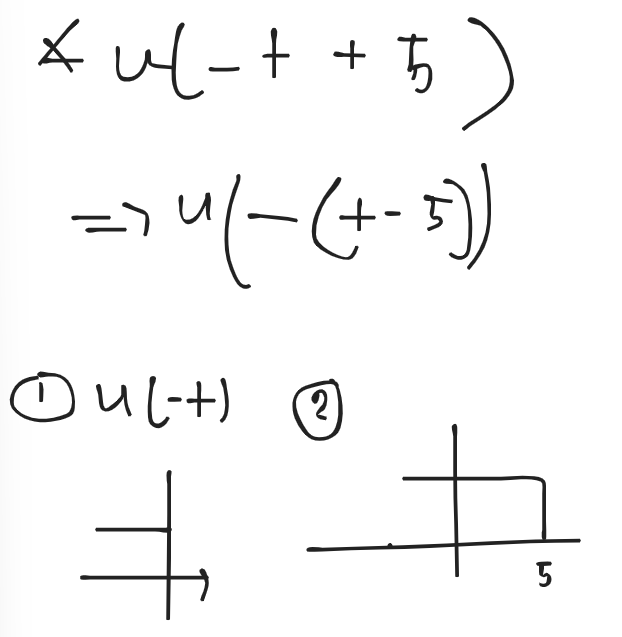
Time Shifting Operation
f(t) is be given. f(t±t0)=?
t0 is a constant
+ → advance : Shift the signal towards left by t0
− → delay : Shift the signal towards right by t0
Amplitude doesn’t change for shifting
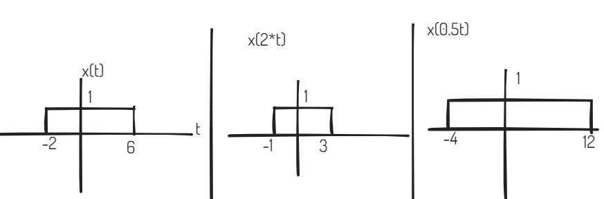
Time Scaling Operation
x(t) is given. f(αt)=?
α : scaling factor
α>1 → Signal Compression (Increasing Speed) : Divide the existing limit by α
α<1 → Signal Expansion (Decreasing Speed) : Divide the existing limit by
Amplitude doesn’t change for this operation
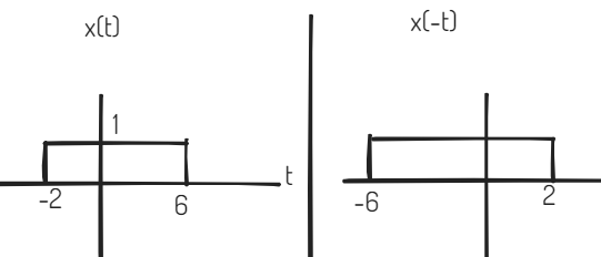
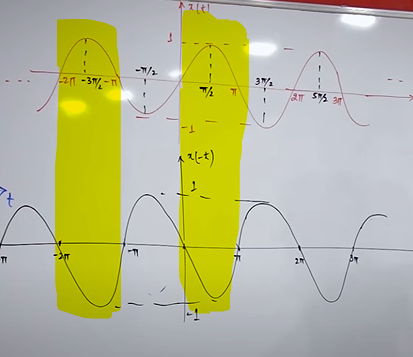
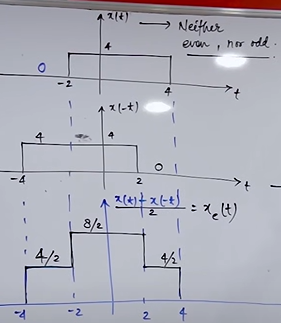
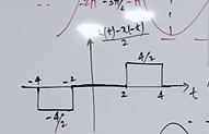
Time Reversal or folding Operation
x(t) is given. x(−t)=?
The sign of the limit will be changed
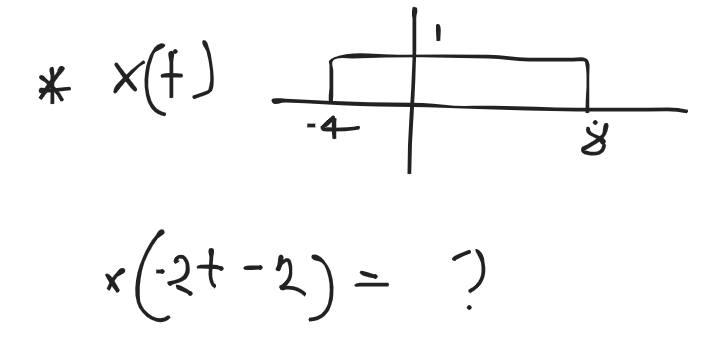
Example on Operation:
Elementary Signals
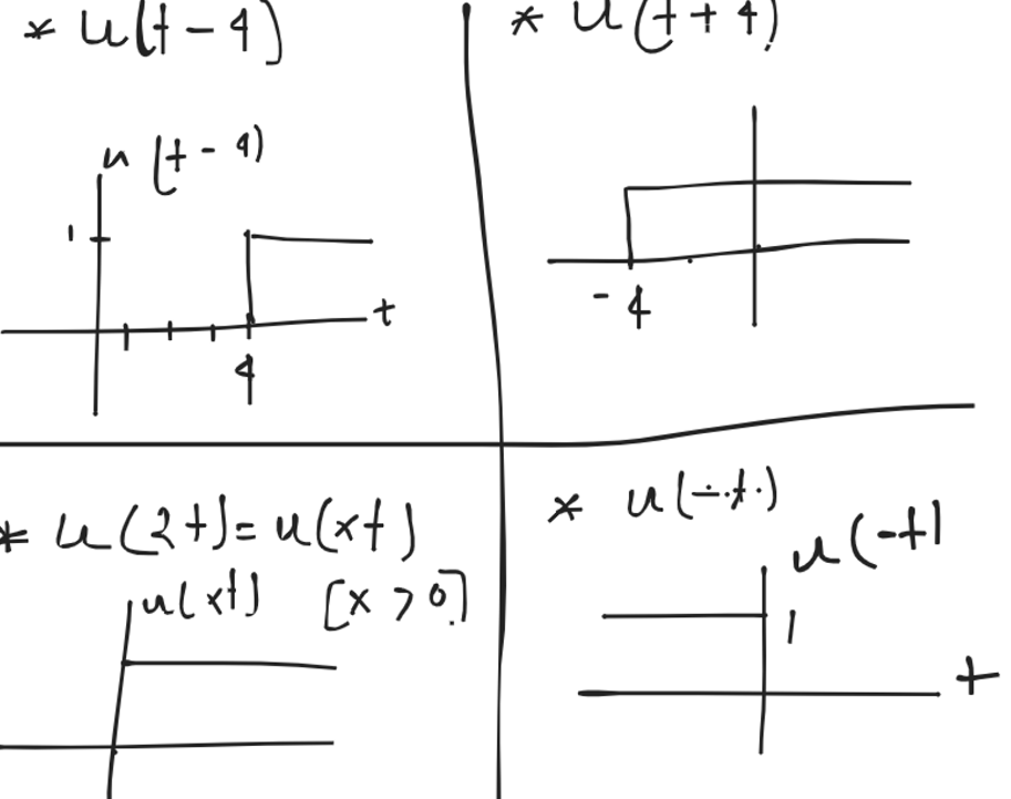
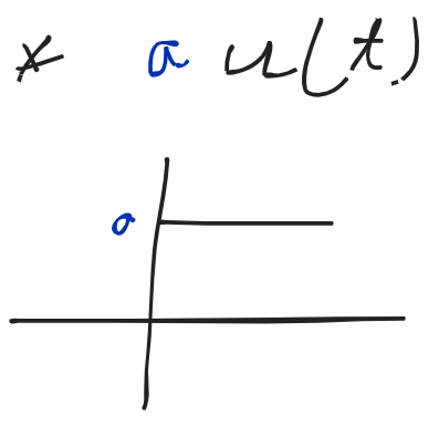
Unit Step Signal
Also known as Heaviside Step Function
Unit step function is denoted by u(t)
u(t)={10t≥0t<0
Amplitude = coefficient of u(t)
Non-Causal Signal∗Unit Step Function = Causal Signal
Operations on Unit Step Signal:
Example:
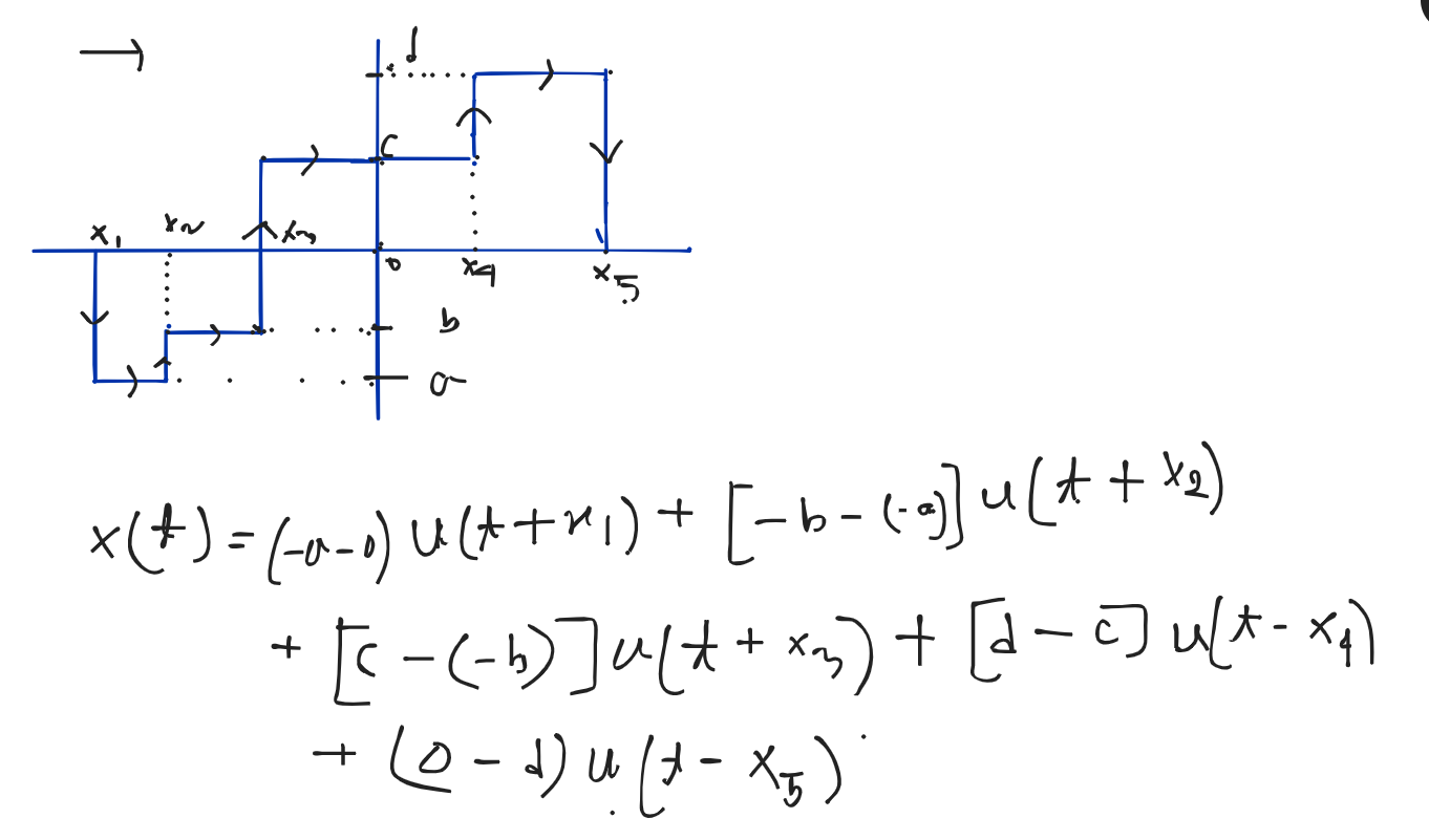
Expressing by unit step function
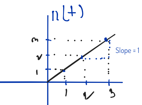
Unit Ramp Signal
r(t)={t0t≥0t<0
Slope = Coefficient of r(t)
r(t)=t⋅u(t)
dtdr(t)=u(t)
dtd[A⋅r(t)]=A⋅u(t)
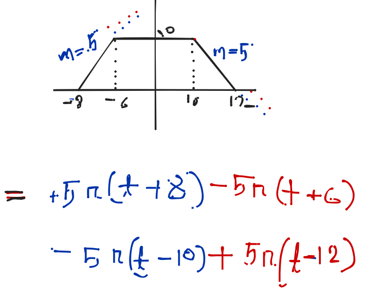
Expressing into Ramp Signal
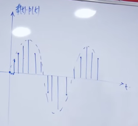
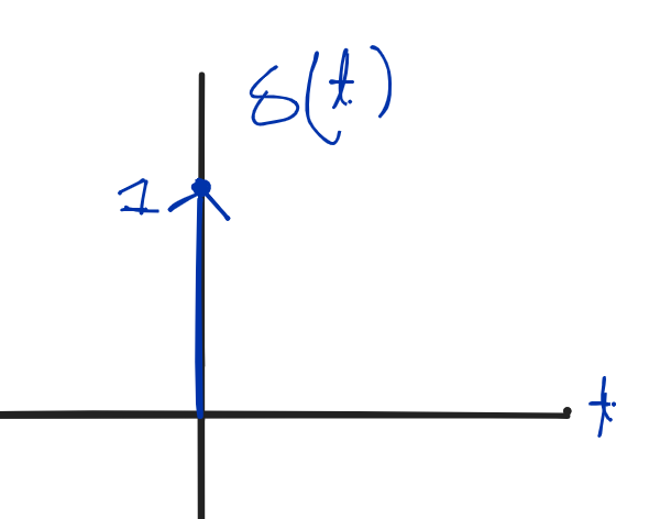
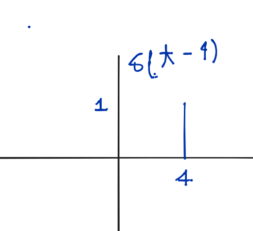
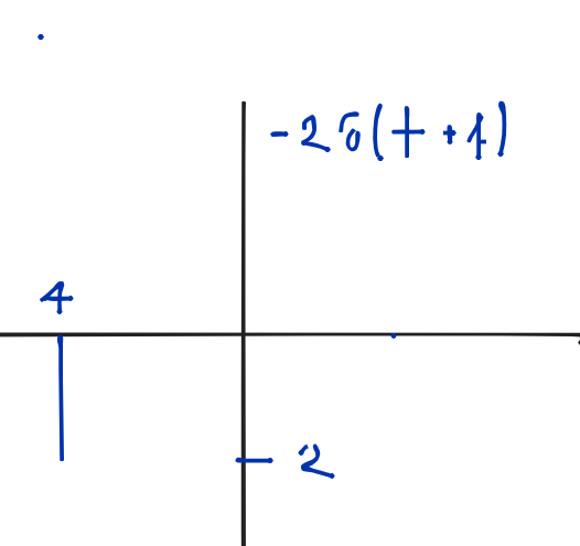
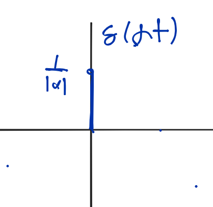
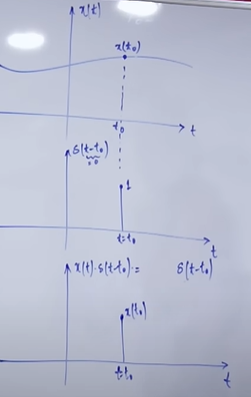
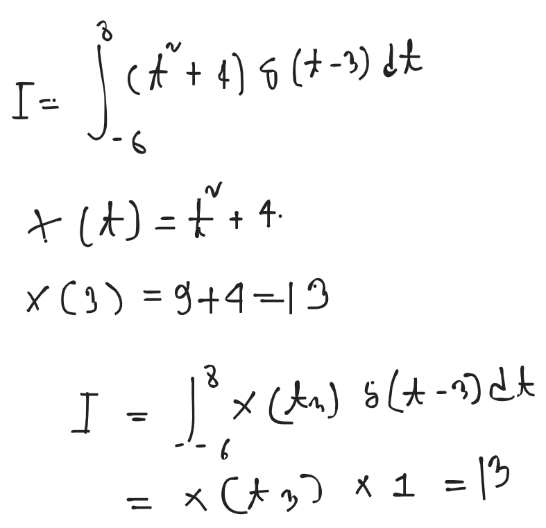
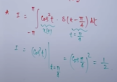
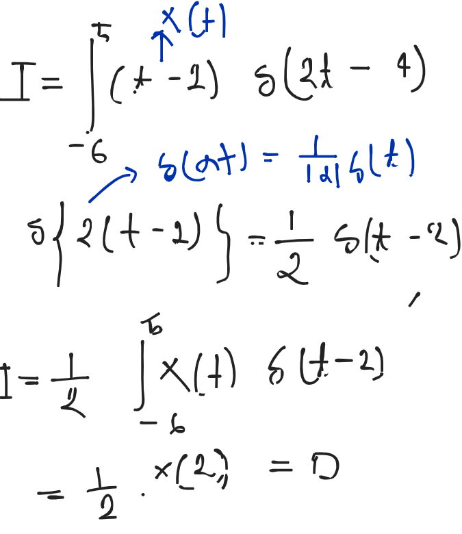
Impulse Function
An ideal impulse signal is a signal that is zero everywhere but at the origin (t = 0), it is infinitely high. Although, the area of the impulse is finite.
δ(t)={10t=0t=0
A⋅δ(t), Here A is the area of this impulse function.
A signal is said to periodic, if it satisfies following two properties
It must be exist for −∞≤t≤∞
It must repeat itself after some constant amount of time T, which is called Fundamental Time Period
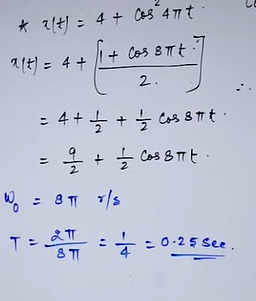
T=w02π
w0= Fundamental frequency rads−1=2πf
T=f1
Frequency must be real number. If frequency is not real number, it’s not periodic.
Types
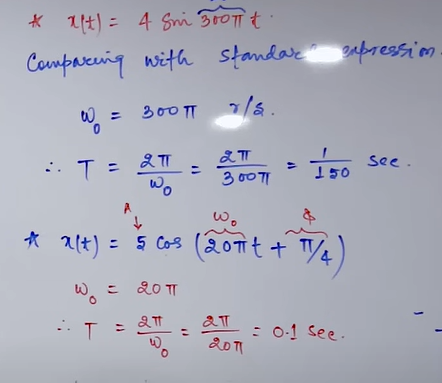
Sinusoidal Signals
Representation
x(t)=Asin(w0t+θ)
A= Amplitude
w0t= Phase Angle
θ=Phase shift (+ → Advance, - delay)
dtd(Phase)=dtd(w0t)=w0=freequency
Shifting effect doesn’t effect on periodicity, T
x(t±kT)=x(t)
Comparing with x(t)=Asin(nπt+θ), if t is not square root of t, then the signal must be periodic.
Combination of periodic signals
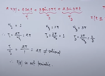
x(t)=Asin(w0t)+Bcos(w1t)+Csin(w2t)+....
x(t) will be periodic if ratio of individual time period is a rational number
Rational Number
Can be expressed by qp. p,q are co-prime.
The value of qp should terminating or repeating decimal. Example : 3.3333.., 2.5, 5.20202020..
Example:T1T2=T2T3=T3T1=RationalNumber
Time Period of Resultant Signal T=LCM(T1,T2,....)
Frequency of Resultant Signal w0′=GCD(w0,w1,....)
If all w0,w1,... have π, then it is periodic. Or if all w0,w1,.... haven’t π, it is periodic too. If some of them have π and rest of them not, then it isn’t periodic.
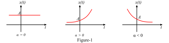
DC/Constant Signal : independent from time. It doesn’t effect on frequency, time. So, it is not countable.
4 is a constant Signal
Energy and Power Signals
Energy Signals
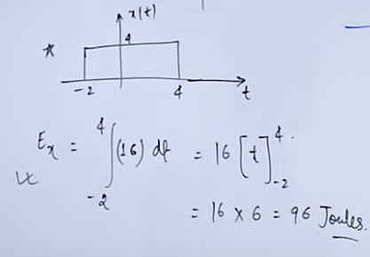
Energy of x(t) is given as
Ex=t→∞lim∫−2T2T∣x(t)∣2dt[No need to take lim if the signal is aperiodic]
if 0<Ex<∞ (Finite), then x(t) is said to be EnergySignal.
Example:
(i)x(t)=e−4t⋅u(t)Ex=∫−∞∞[e−4t⋅u(t)]2dt=∫0∞e−8tdt[u(t) exists only 0 to ∞]=81
When a signal x(t) will be energy signal
If x(t) is existing for infinite direction and decreasing in value.
t→∞limf(t)=0
If x(t) exists for finite direction and value of x(t) is finite finite at all points, x(t) is energy signal.
Power Signals
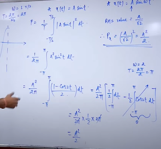
PowerSignal of x(t) is given as
Px=T→∞limT1⋅E=T→∞limT1∫−2T2T∣x(t)∣2dt=T→∞lim2T1∫−TT∣x(t)∣2dt[No need to take lim if the signal is aperiodic]
If 0<Px<∞ (Finite), then x(t) is said to be Power Signal
Power=RMS2
x(t)=Asinwt,RMS=2A,P=RMS2=2A2
When a signal will be Power Signal
All periodic signal are power signal but converse is not true
If x(t) is not a periodic signal and follows the conditions
t→∞limf(t)=0
t→∞limf(t)=∞
A signal can’t be Energy and Power Signals together.
If Ex is finite, then Px is Zero . Vice-Versa.
Operations
Time shifting has no effect on power and energy of signal.Powerx(t)=Powerx(t−2T)Energyx(t)=Energyx(t−4)
Time Scaling doesn’t effect on Time Periodic but in Time period, Energy.
For x(t)T,Exx′(t)=x(αt),T′=αT,Ex′=αEx
Power remains same.
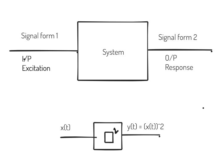
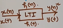
Systems
System is a interconnection of different physical components which is used to convert one form of signal to others.
Example:
Properties of Systems
Static and Dynamic System
Static
Memoryless
if present o/p depends on only present i/p
Dynamic
With Memory
if present o/p depends on past or future i/p
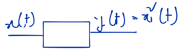
y(2)=x(22)=x(4), t=2’s output depends of t=4. That means present o/p depends on future i/p;
Causal, Noncausal, Anticausal
Causal
Present o/p depends on
present i/p or
Present + Past i/p
Static system are always causal
h(t)=0t<0h[n]=0t<0
Noncausal
Present o/p depends on
present + future or
present + past + future or
past + future
h(t)=0,t<0h[n]=0,t<0
y[n]=x[n2]y[0]=x[0]y[1]=x[1] depends on presenty[2]=x[4] depends on future
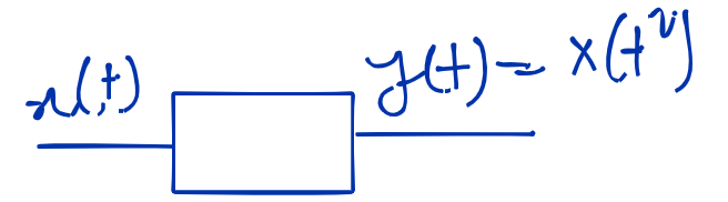
Anticausal
Present o/p depends on
only future i/p
y(t)=x(t2+1)y(0)=x(1)y(−1)=x(0)
depends on only future
h(t)=0t>0h[n]=0t>0
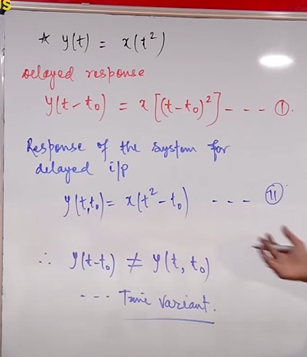
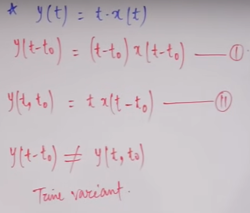
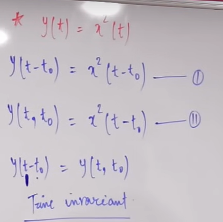
Time variant and Invariant System
Time Invariant
If time shift in i/p results identical time shift in o/p without changing the nature of the output.
To check
Find y(t) delay, y(t−t0), replace t with t−t0
Find x(t−t0)=y(t,t0), response of the system for delayed i/p
y(t,t0)=write the y(t) just add/minus t0
if y(t−t0)=y(t,t0), it is time variant.
For a system to be time invariant
There must not be any scaling in x(t) or y(t)
Coefficient must not function of time
Any extra term except x(t) or y(t) must be zero or constant
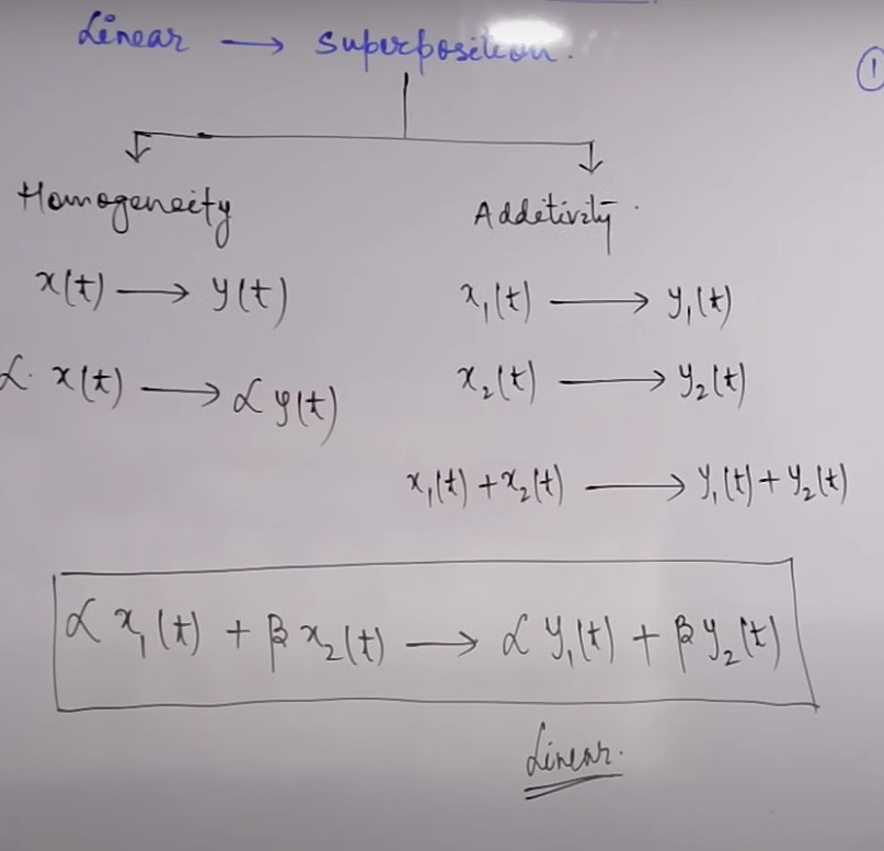
Linear and Nonlinear System
Linear
If the system follows principle of superposition
To check linearity
Graph between output and input must be throughout a straight line passing through origin without having saturation or dead zone
If system is represented by a linear differential equation, then the equation must be linear.
System must be follow zero input zero output criteria.
x(t)→y(t)αx(t)→αy(t)0=0,α=0
Mathematical way to prove a system is linear or not
Given, x(t)→y(t)=tx(t)
x1(t)→y1(t)=tx1(t)
x2(t)→y2(t)=tx2(t)
y3(t)=y1(t)+y2(t)=t(x1(t)+x2(t))...(1)
x3′(t)=x1(t)+x2(t)
y3′(t)=tx3(t)=t(x1(t)+x2(t))...(2)
(1)=(2), it follows the additivity.
αx(t)→αy(t)=αtx(t)
y′(t)=t[αx(t)]=αtx(t)...(3)
αy(t)=αtx(t)...(4)
(3)=(4),it follows the homogeneity rule
Checking homogeneity and additivity at once
x(t)→y(t)αx1(t)+βx2(t)→αy1(t)+βy2(t),the system will be lineary
Given, y(t)=x[sint]
y1(t)=x1[sint],y2[t]=x2[sint]
y3(t)=αy1(t)+βy2(t)=αx1(sint)+βx2(sint)
x3′(t)=αx1(t)+βx2(t)
y3′(t)=x3′(sint)=αx1(sint)+βx2(sint)
Invertible and Non-invertible
Invertible
If distinct input produces distinct outputs
if input can be determined by observing output
a inverse system can be design, overall gain = 1
Stable and Unstable System
Stable
Follows bounded input bounded output(BIBO)
The output of the system must be bounded for bounded input
0≤∣x(t)∣<∞, then 0≤∣y(t)∣<∞
BIBO implies that impulse response must tend to zero , as time tends to infinity.
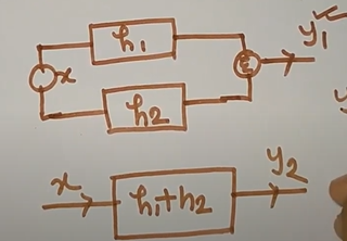
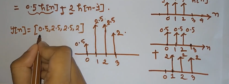
Summing of the outputs of of two systems is equivalent to a system with an impulse response equal to the sum of the impulse response of the two individual system.
y1=y2
y1=x∗h1+x∗h2
y2=x∗(h1+h2)
Hence, x∗h1+x∗h2=x∗(h1+h2)
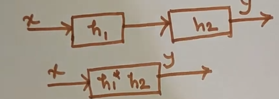
Associative Property
The change of order of the cascaded system will not affect the response.
y=x∗(h1∗h2)=(x∗h1)∗h2
LTI System with and without memory
Memoryless → Output(t) → input(t), Current output depends on only current input
DTS: h[n]=0 for n=0
CTS: h[t]=0 for t=0
Otherwise, with memory.
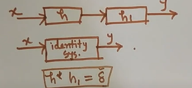
Invertibility of LTI System
A system S is invertible if and only if there exists an inverse system S−1 such that S−1 is an identity system.
h∗h1=δ
Causality Property
DTS:h(n)=0,n<0
CTS: h(t)=0,t<0
Stability Property
∑k=∞∞∣h(k)∣<∞, for DTS
∫−∞∞∣h(t)∣<∞, for CTS
Check Causality and Stability for h(n)=21nu(n) (DTS : Discrete Time Signal)
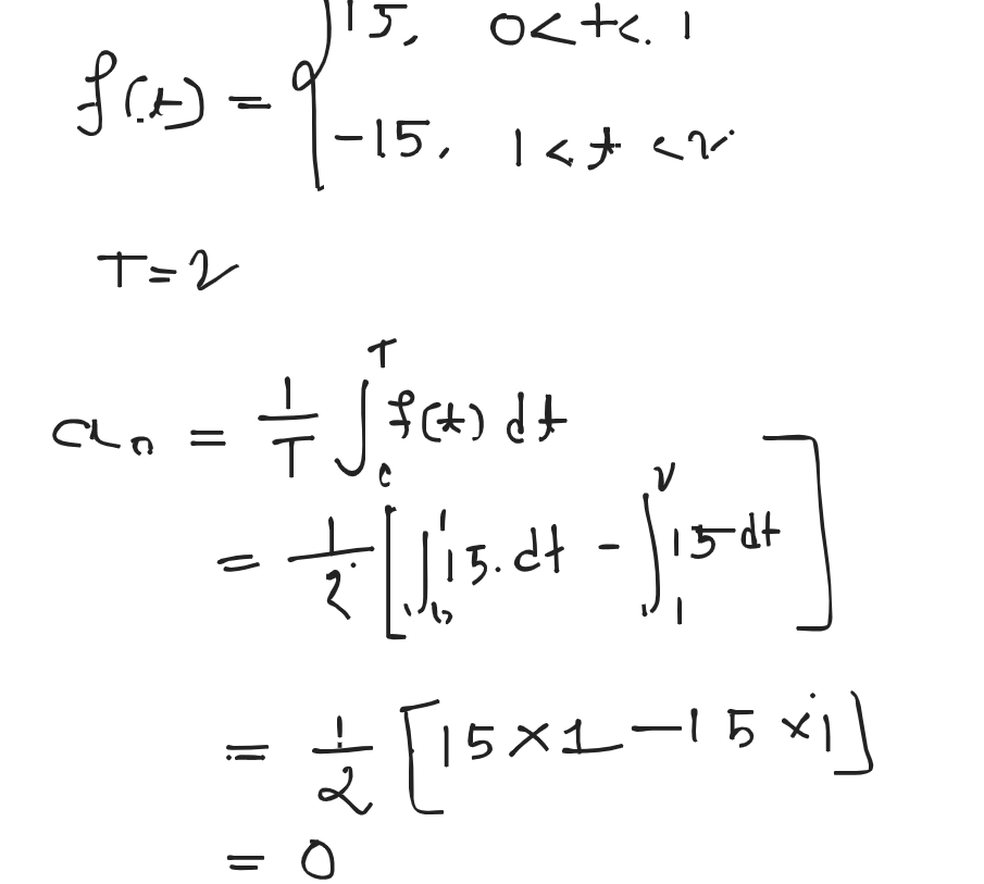
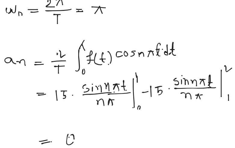
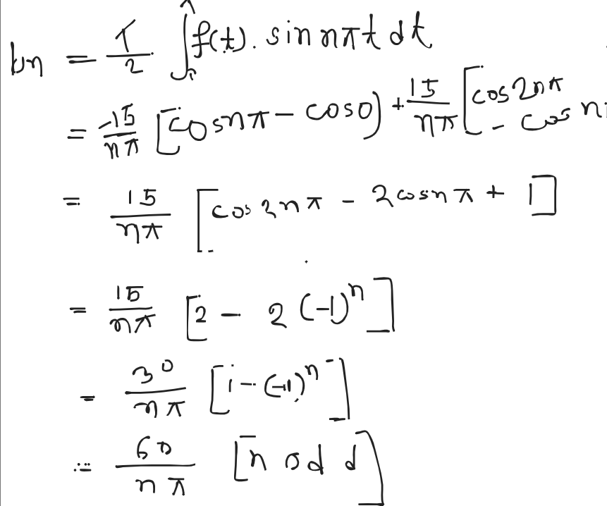
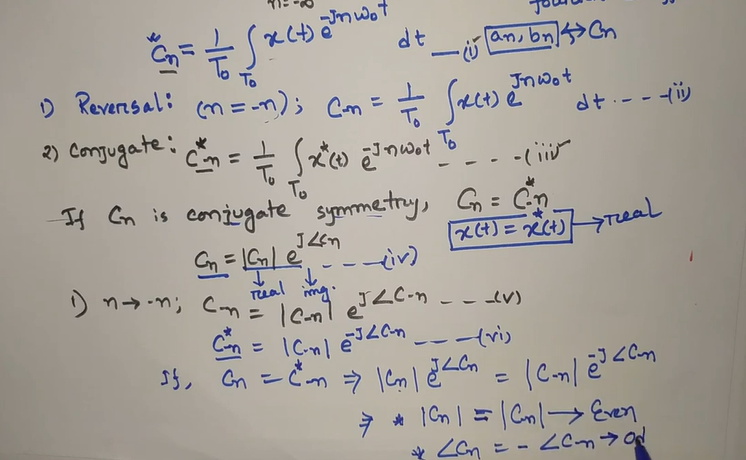
Fourier Series is a sum that represents a “periodic function” as a sum of sine and cosine waves in terms of their harmonics.
x(t)=x(x±T), T : Time period, x(t) is periodic.
Frequency, f=noofcycle/sec / rate of change
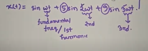
Harmonics
3rd Harmonics will dominant 2nd one because it’s magnitude is greater than the 2nd one. (9 > 5)
Dirichlet conditions of Fourier Series
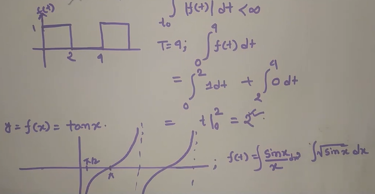
Function f(t) is single valued everywhere.
f(x)=x2;
For every x there is only one f(x)ory
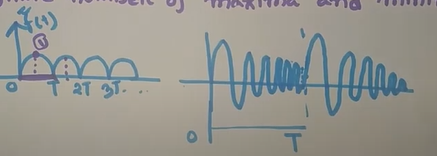
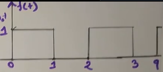
Function has a finite number of discontinuities in any time period.
Function has a finite number of maximum and minimum in any time period.
Signal should be absolutely integrable in any time period.
∫t0t0+T∣f(t)∣dt<∞
Why sineandcosine are special to Fourier Series ?
The Fourier series uses cosine and sine functions because they form a complete set of orthogonal functions, meaning they are independent and can be used to represent any periodic function