DBMS
| Created by | Borhan |
|---|---|
| Last edited time | |
| Tag | Year 3 Term 1 |
Resources
Introduction
Database: The collection of data, usually referred to as the database, contains information relevant to an enterprise.
Database-management System: A database-management system (DBMS) is a collection of interrelated data and a set of programs to access (retrieve, insertion, deletion, update) those data.
Goal of DBMS
- Providing a way to store and retrieve database information that is both convenient (easy) and efficient (quick, correct).
- Ensuring the safety of the information.
File System:
Disadvantage of File System
- Data redundancy and inconsistency
- Difficulty in accessing data
- Data Isolation
- Integrity Problem: applying constraints
- Atomicity Problem
- Concurrent-Access Anomalies
- Security Problem
Database Architecture
Schema: The overall design of the database is called the database schema.
Instance: The collection of information stored in the database at a particular moment is called an instance of the database.
Database Language
- Data-Definition Model (DDL): for Schema
- Data-Manipulation Language (DML) : for Instance
- Procedural DMLs: Require a user to specify what data are needed and how to get this data
- Non-procedurals (Declarative): Require a user to specify what data are needed without specifying how to get those data. Example: SQL
Database Users and Admins
- Naive users : Accessing database without even knowing
- Application programmers: Accessing databasing using some statements
- Sophisticated users: Accessing database using query
- Specialized users: Database design or who makes DBMS
- Database Administrator: Maintaining database, authentication, authorization, clean up
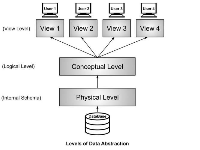
View of Data
- Physical Level: Describes how data is physically stored in the database. The Database Administrators(DBA) decide that which data should be kept at which particular disk drive, how the data has to be fragmented, where it has to be stored etc. It ensures efficient data storage and retrieval.
- Logical/Conceptual Level: Describes the logical structure of the entire database. It focuses on designing how data is organized conceptually.
- View Level: Defines how data is viewed by specific users or applications. It enhances security and ease of access by showing only relevant data to users.
3 Levels of Data Abstraction: Data Abstraction refers to the process of hiding irrelevant details from the user.
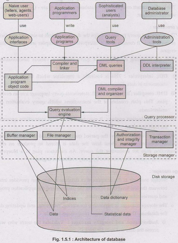
Database System Structure
The functional components of a database system
- Storage manager: The storage manager is responsible for storing, retrieving, and updating the database
- Query processor components: The interactive query processor helps the database system to simplify and facilitate access to data
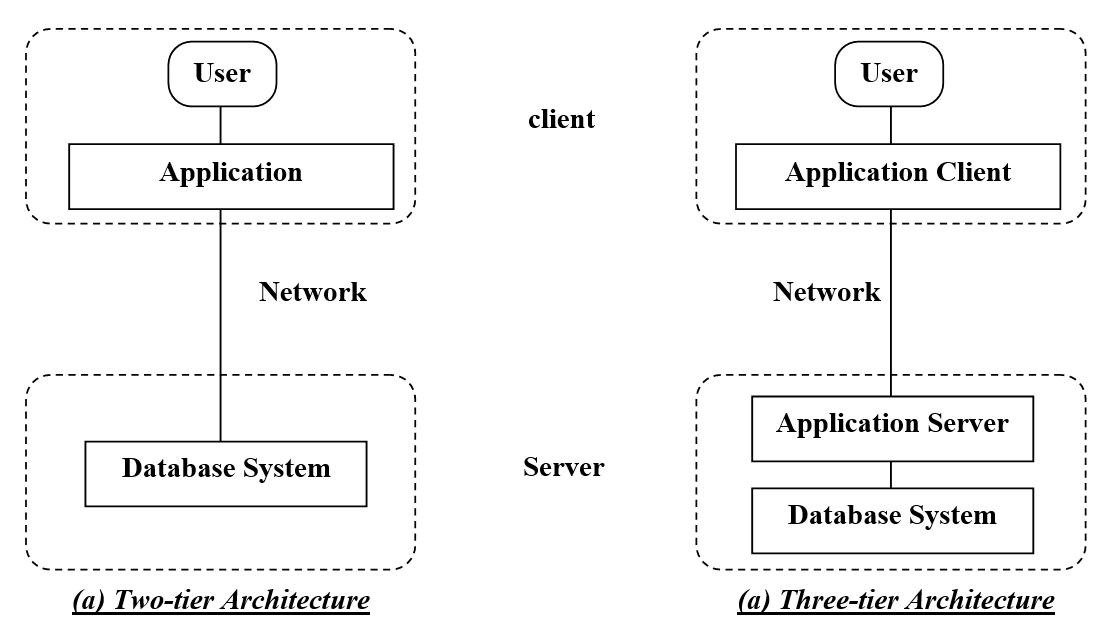
2-tier and 3-tier database
Database Designing
Data Models: A collection of conceptual tools for describing data, data relationship, data semantics and consistency constraints.
Data Models types:
- Entity-Relationship Model: The entity-relationship (E-R) data model consists of collection of basic objects, called entities and of relationship among these objects.
- Relational Model: The relational model is a collection of tables to represent both data and the relationship among these data.
- Object-oriented data model
- Network data model
- Hierarchical data model
Database design:
- Requirement Analysis
- Conceptual Database Design: E-R Model
- Schema Refinement: Finetuning the relations, Normalization
- Logical database design: Relational Modelling
- Physical database design: Decide the data structure to store database (storage), indexing
- Security Design: Authentication, authorization
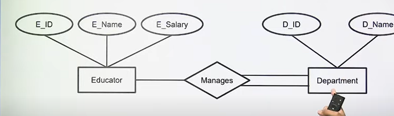
The Entity-Relationship Model
The Entity-Relationship data model consists of collection of objects called entities and of relationship among these objects.
Entity: Object in the real world that is distinguishable from another object.
Entity-set: A collection of similar entities called an entity set.
Attribute: An entity is described using a set of attributes.
Domain: A unique set of values permitted for an attribute.
Relationship: An association among two or more entities.
Relationship-set: A set of similar relationship.
Key: An attribute or set of attributes whose values can uniquely identify an entity in a set.
E-R Diagram: An Entity-Relationship (E-R) Diagram is a visual/graphical representation of the data model for a system. It uses specific symbols to depict the entities relationships , and attributes in a database.
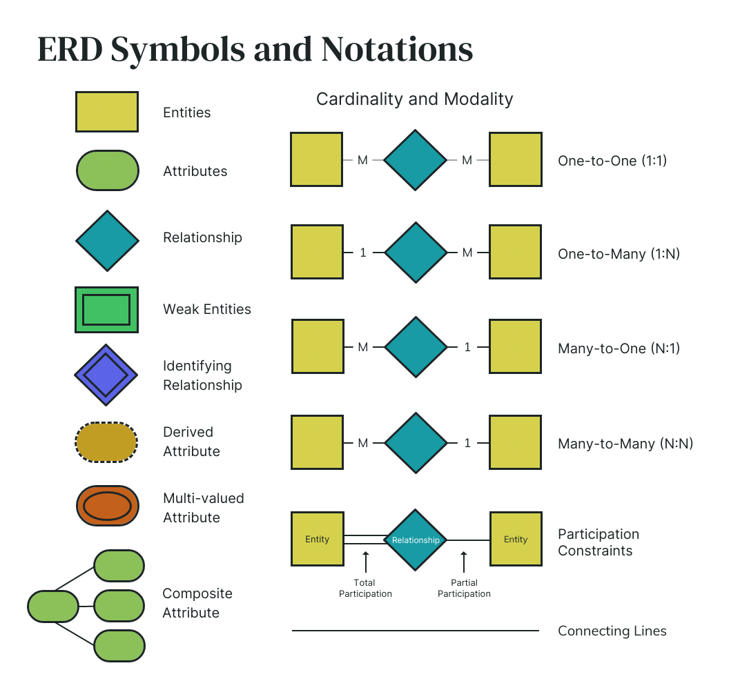
Types of Relationships
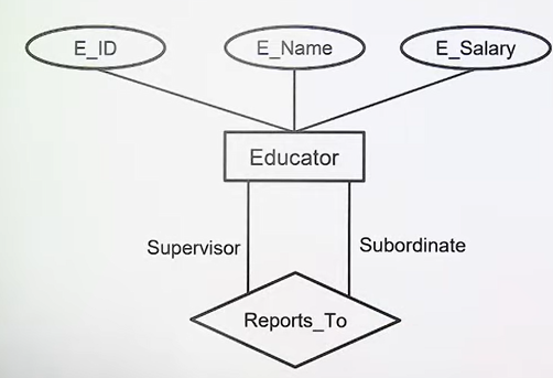
- Unary: Relationship between entities of same entity set.
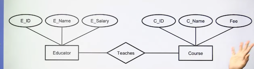
- Binary: Relationship between entities of two entity-sets.
- Ternary: Relationship between entities of three entity sets.
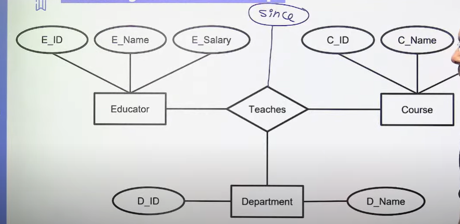
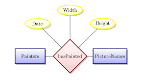
Descriptive attribute: Attribute of relationship.
Mapping Cardinality: The maximum number of relationship in which an entity can participate.
- One to One:
- One to Many:
- Many to One:
- Many to Many:
Participation Constraints: Specifies the presence of an entity when it is related to another entity in a relationship type.
- Total Participation: Every instance of an entity must participate in the relationship.
- Partial Participation: Only some instances of an entity participate in the relationship.
| Aspect | Total Participation | Partial Participation |
|---|---|---|
| Definition | Every instance of an entity must participate in the relationship. | Only some instances of an entity participate in the relationship. |
| Requirement | Mandatory for all instances to be associated. | Optional; not all instances need to be associated. |
| Representation in E-R Diagram | Represented by a double line connecting the entity to the relationship. | Represented by a single line connecting the entity to the relationship. |
| Example | In a marriage relationship, every spouse must participate. | In a course enrollment relationship, not all students need to enroll in courses. |
| Use Case | Used when an entity’s existence depends on its participation in the relationship. | Used when an entity can exist independently of the relationship. |
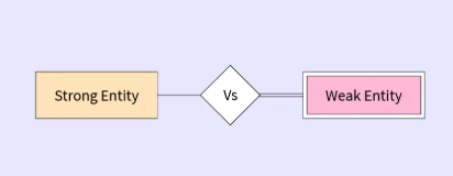
Weak and Strong Entities
- Weak Entity: A weak entity is an entity that cannot be uniquely identified by its attributes alone.
- Strong Entity: A strong entity is an entity that can be uniquely identified by its own attributes without relying on other entity.
| Aspect | Weak Entity | Strong Entity |
|---|---|---|
| Definition | An entity that cannot be uniquely identified by its own attributes alone and requires a foreign key from another entity (its owner). | An entity that can be uniquely identified by its own attributes without relying on any other entity. |
| Key Attribute | Does not have a primary key of its own. Uses a composite key (combination of its own partial key and the primary key of the related entity). | Has a primary key that uniquely identifies each instance. |
| Relationship Dependency | Always exists in a dependent relationship with a strong entity. | Exists independently without any dependency on other entities. |
| Representation in E-R Diagram | Represented by a rectangle with a double border. | Represented by a rectangle with a single border. |
| Relationship Type | Connected via a strong (identifying) relationship with the owner entity, represented by a double diamond. | Connected via a regular relationship, represented by a single diamond. |
| Example | A dependent entity in an insurance database where each dependent needs an associated policyholder (strong entity). | A customer entity in a banking database that can exist independently. |
| Use Case | Used when the entity relies on another for identification (e.g., OrderItem in an Order system). | Used when the entity stands alone and has its own identifier (e.g., Product, Employee). |
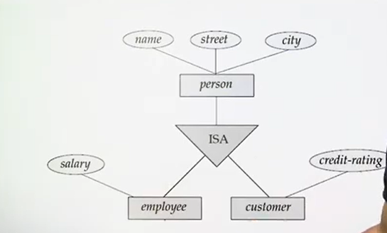
Extended E-R Features
- Specialization
- Generalization
- Higher-and-lower-level entity sets
- Attribute inheritance
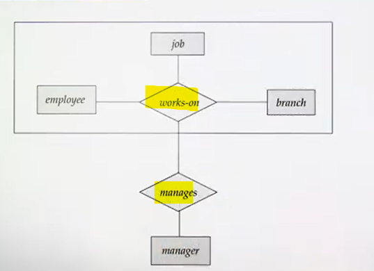
- Aggregation
Specialization: The process of designating subgroupings withing an entity sets is called specialization.
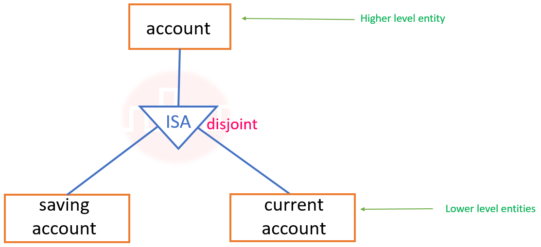
Specialization types:
- Disjoint: An entity instance can belong to only one of the specialized subclasses.
- Overlapping: An entity instance can belong to multiple specialized subclasses simultaneously.
Higher and lower level entity sets:
Higher-level entity sets: A generalized entity set that represents common attributes of multiple specialized entities.
Lower-level entity sets: A specialized entity set that represents a subset of the higher-level entity with additional, specific attributes.
| Aspect | Higher-Level Entity Set | Lower-Level Entity Set |
|---|---|---|
| Definition | A generalized entity set that represents common attributes of multiple specialized entities. | A specialized entity set that represents a subset of the higher-level entity with additional, specific attributes. |
| Abstraction Level | Represents a broader and more abstract entity. | Represents a more specific and detailed entity. |
| Relationship | Serves as the parent entity in a generalization/specialization hierarchy. | Serves as the child entity derived from the higher-level entity. |
| Attributes | Contains attributes common to all related lower-level entities. | Contains attributes inherited from the higher-level entity plus unique attributes. |
| Example | Vehicle (common attributes: Vehicle ID, Model) | Car, Bike, Truck (specific attributes: Number of Wheels, Fuel Type) |
| Use Case | Useful for representing common characteristics in different subcategories. | Useful for distinguishing between various categories with unique characteristics. |
Generalization : This commonality can be expressed by generalization, which is a containment relationship that exists between a higher-level-entity-set and one or more lower-level entity sets.
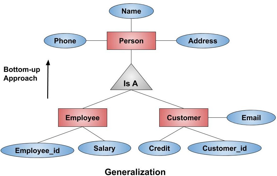
- Total generalization/specialization: Each higher-level entity must belong to a lower-level entity set.
- Partial generalization/specialization: Some higher-level entities may not belong to any lower level entity.
Attribute Inheritance: Attribute inheritance refers to the concept in generalization and specialization where lower-level entities (subclasses) inherit the attributes of their higher-level entity (superclass).
Aggregation: Aggregation is an abstraction used in Entity-Relationship (E-R) diagrams to represent a relationship between a relationship and another entity.
Attributes
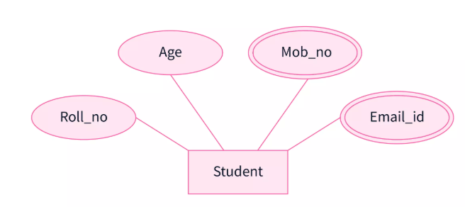
Single vs Multivalued Attributes
| Aspect | Single-Valued Attribute | Multivalued Attribute |
|---|---|---|
| Definition | An attribute that can hold only one value for each entity instance. | An attribute that can hold multiple values for each entity instance. |
| Number of Values | Stores one value per entity instance. | Stores multiple values per entity instance. |
| Complexity | Simpler and requires less storage. | More complex and requires additional storage or normalization. |
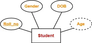
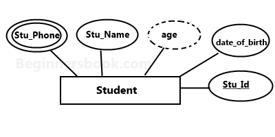
| Representation in E-R Diagram | Represented as a single oval. | Represented as a double oval. |
| Example | Phone Number of an entity Customer where only one phone number is allowed. | Phone Number of an entity Customer where multiple phone numbers are allowed. |
| Use Case | Used when each instance of an entity has exactly one value for the attribute (e.g., Date of Birth). | Used when an entity instance can have multiple values for the attribute (e.g., Email Addresses, Skills). |
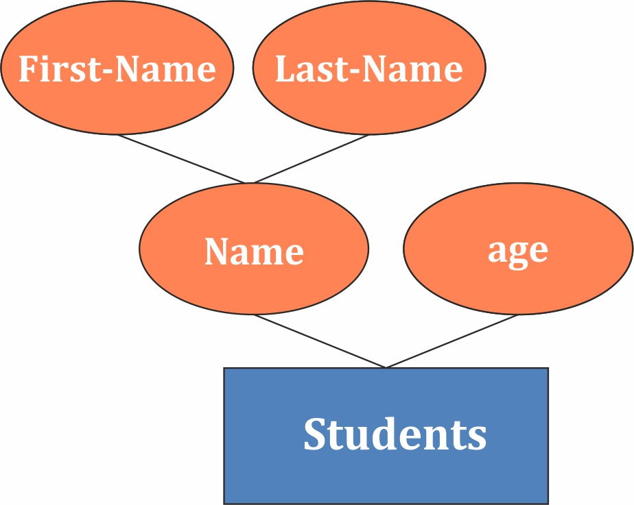
Simple vs Composite Attributes
| Aspect | Simple Attribute | Composite Attribute |
|---|---|---|
| Definition | An attribute that cannot be divided into smaller parts or components. | An attribute that can be divided into smaller sub-parts or sub-attributes. |
| Components | Contains one single value for each entity instance. | Composed of multiple sub-attributes, each representing a part of the whole. |
| Complexity | Less complex and represents a single data element. | More complex as it represents a combination of smaller attributes. |
| Example | Age, Salary, Phone Number (if considered as a single value) | Full Name (composed of First Name and Last Name), Address (composed of Street, City, Zip Code) |
| Use Case | Used when only one value is needed to describe the entity's property. | Used when the attribute needs to be described using multiple components. |
Given vs Derives Attributes
| Aspect | Given Attribute | Derived Attribute |
|---|---|---|
| Definition | An attribute that stores actual data provided by the entity or its relationship. | An attribute that is calculated or derived from other existing attributes in the system. |
| Data Source | Comes from direct input or stored data in the database. | Does not directly store data, but is computed based on other attributes. |
| Representation in E-R Diagram | Represented by a single oval. | Represented by a dashed oval. |
| Example | Date of Birth, Employee ID | Age (derived from Date of Birth), Total Salary (derived from Basic Salary + Bonus) |
| Use Case | Used for attributes that are explicitly stored and provided for the entity. | Used for attributes that are inferred or calculated, not directly stored. |
Prime vs Non-prime attribute
| Aspect | Prime Attribute | Non-prime Attribute |
|---|---|---|
| Definition | An attribute that is part of a candidate key of an entity. | An attribute that is not part of any candidate key of an entity. |
| Key Role | Essential for uniquely identifying an entity. It helps define the primary key. | Does not directly contribute to the entity's unique identification. |
| Example | In a Student entity, Student ID and Email could be candidate keys. Student ID would be a prime attribute. | In the same Student entity, Name, Address, and Phone Number would be non-prime attributes. |
| Use Case | Used when attributes are essential for distinguishing between different instances of an entity. | Used when attributes are additional or descriptive information about the entity. |
Relational Model
The Relational Model is a data model used to organize data into tables (relations) consisting of rows (tuples) and columns (attributes). It was introduced by E.F. Codd in 1970 and forms the basis for most modern relational database management systems (RDBMS).
Relation: The main construct for representing data in the relational model is a relation, which is a table.
Attribute/Field: Attributes are used to describe relations. Columns of relations are attributes.
Tuple/Record: A row in a relation.
Instance: Snapshot of the data in the database at a given instant in time.
Database Schema: Logical design of database. Example: Reation_name(attribute1, attribute2)
Domain: A unique set of values permitted for an attribute.
Domain Constraint: Specifies an important condition that we want each instance of relation to satisfy,
Degree/Arity: Number of attributes in a relation.
Cardinality: Number of tuples in a relation.
Relational Databases: A relational databases is a collection relations.
Keys: An attribute or set of attributes which value can uniquely identify a tuple in a relation.
Types of keys
- Super Key: A super key is a set of one or more attributes in a relation (table) that can uniquely identify each tuple (row) in that relation.
- Candidate Key: A candidate key is a minimal set of attributes in a table that can uniquely identify each tuple (row) in the relation. It contains the smallest possible number of attributes required for unique identification.
- Primary Key: A primary key is a specific type of candidate key chosen to uniquely identify each tuple (row) in a relational database table. Primary keys cannot contain
NULLvalues.
- Alternate Key: All candidate keys apart from primary key,
- Foreign Key: A foreign key is an attribute (or a set of attributes) in a table that references the primary key in another table. It establishes a relationship between two tables, enforcing referential integrity by ensuring that the value in the foreign key column corresponds to a valid value in the referenced table’s primary key.
Referential Integrity: Referential integrity ensures data consistency between tables by enforcing that a foreign key in one table either matches a primary key in another table..
| Aspect | Super Key | Candidate Key | Primary Key | Alternative Key | Foreign Key |
| Definition | A set of one or more attributes that uniquely identifies each tuple. | A minimal set of attributes that uniquely identifies each tuple. | A selected candidate key used to uniquely identify each tuple. | A candidate key not chosen as the primary key. | An attribute in one table that references the primary key in another table. |
| Uniqueness | Must be unique but can have extra attributes. | Must be unique and minimal. | Must be unique and minimal. | Must be unique and minimal. | May contain duplicate values. |
| Minimality | Not necessarily minimal. | Always minimal. | Always minimal. | Always minimal. | Not required to be minimal. |
| Number per Table | Can have multiple super keys. | Can have multiple candidate keys. | Only one primary key per table. | All candidate keys except the primary key. | Can have multiple foreign keys pointing to different tables. |
| Null Values | Can allow NULL. | Cannot contain NULL (if used as a primary key). | Cannot contain NULL. | Cannot contain NULL (if used as a key). | Can allow NULL. |
| Purpose | Uniquely identifies rows but may have redundant attributes. | Potential keys for identifying rows uniquely. | Enforces entity integrity. | Acts as backup keys if the primary key fails. | Enforces referential integrity between tables. |
| Example | {Student ID, Name}, {Student ID} | {Student ID}, {Email} | {Student ID} | {Email} (if not chosen as primary key). | {Student ID} in the Order table referencing Student ID in the Student table. |
ERD to Relational Model
Many → One
Best solutions:
Many to many relationship : one extra table is needed for relationship information along with the two tables.
One to Many relationship: creates only two tables keep relationship information toward many sides.
One to one relationship: Keep information any of them, no extra table is needed. If only one entity set having total participation then keep relationship information towards total participation table to avoid multiple null tables.
Specialization and generalization: Possible with two tables.
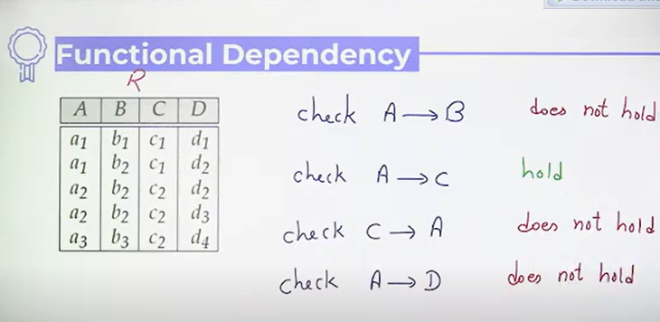
Functional Dependency (FD)
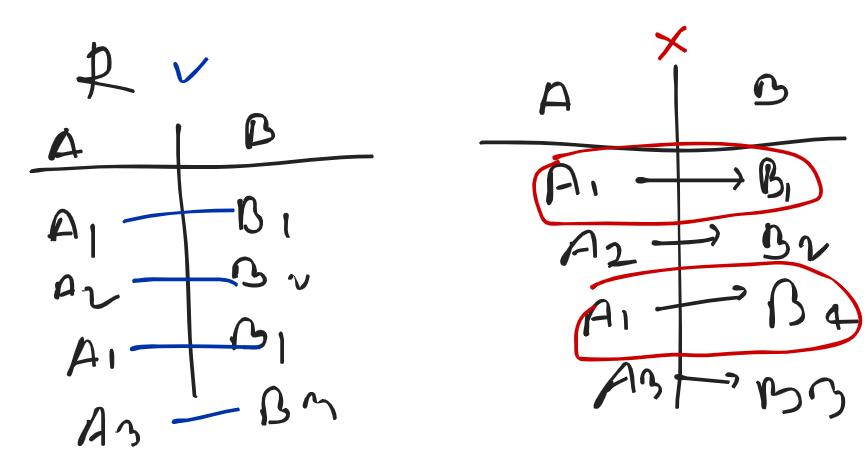
Consider a relation R and 2 attributes A and B
B is functionally dependent on A (denoted by A → B), if each value of A is associated with exactly one value in B in relation.
- Functional dependencies play a key role in differentiating good database design from bad database design.
- A functional dependency is a type of constraint that is a generalization of the notion of key. (By helping of FD, we can say which attribute or attributes gonna be key. )
- X → Y, where X is a set of attributes that can determine the value of Y.
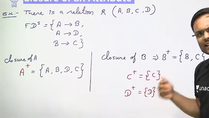
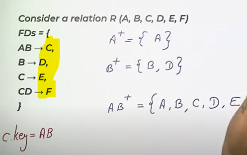
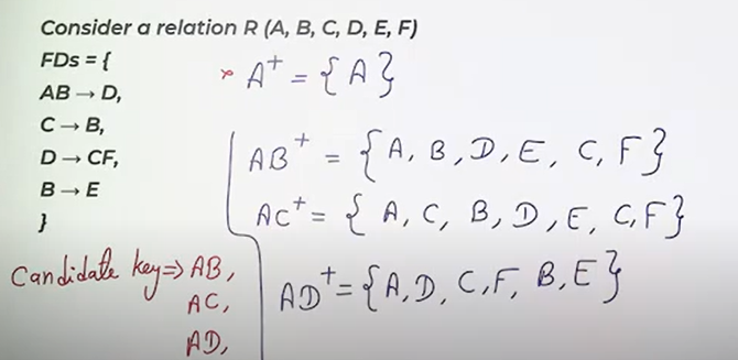
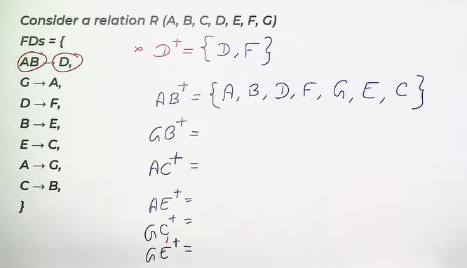
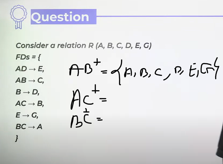
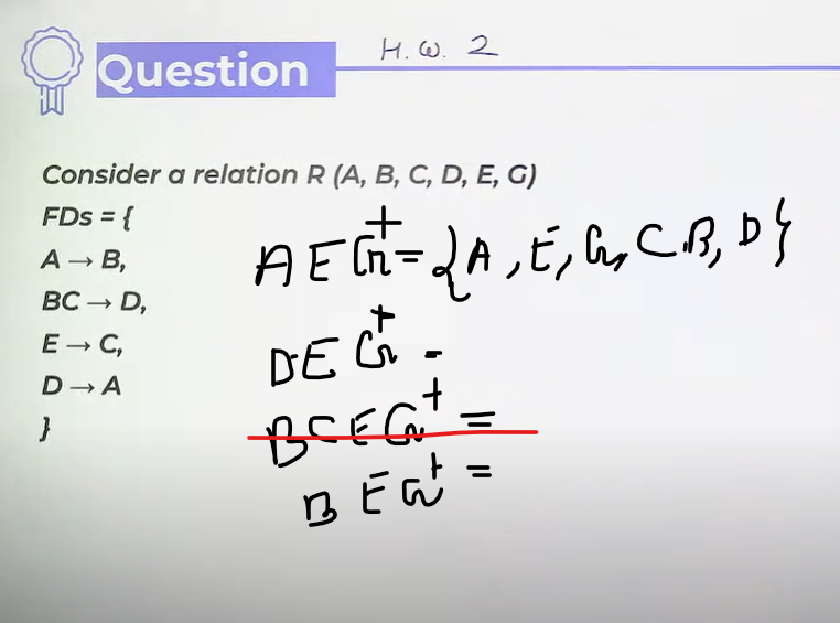
Closure of Attributes: The closure of a set of attributes (denoted as ) is a set of attributes that can be functionally determined by the given set of attributes X in a relation.
Properties
Trivial: Some functional dependencies are said to be trivial because they are satisfied by all relations. (Trivial means obvious) Example: A→ A
Armstrong’s Axioms
- Reflexivity Rule: , if
- Augmentation Rule: If then
- Transitivity Rule: If , , then
Additivity Rules
- Union Rule: If then
- Decomposition Rule: If then and
- Pseudo-transitivity rule: If , then
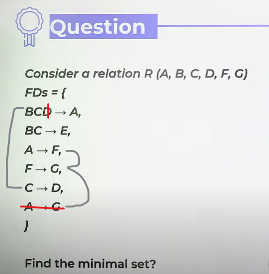
Finding keys from FD
Normalization
Normalization is the process of minimizing redundancy from a relation or set of relations.
Redundancy in relation may cause insertion, deletion and update anomalies.
Essence of Normalization : One relation should have one theme.
Process of Normalization
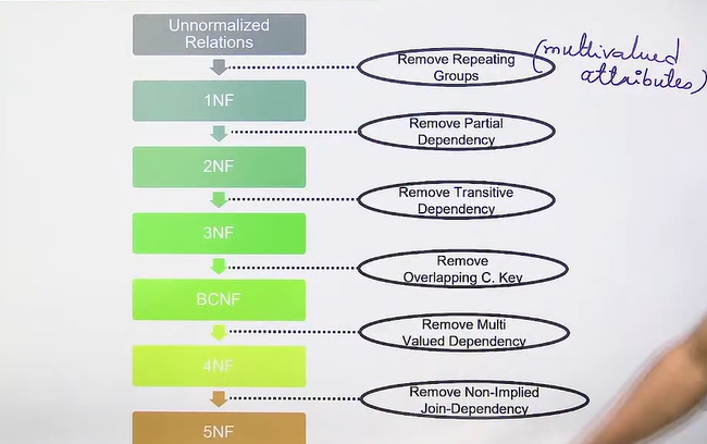
1 NF : 1st Normal Form
A relation R is said to be in 1NF if there are no any multivalued attribute in R.
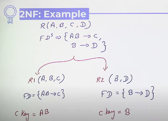
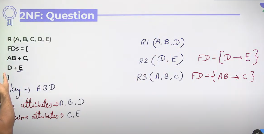
2NF : 2nd Normal Form
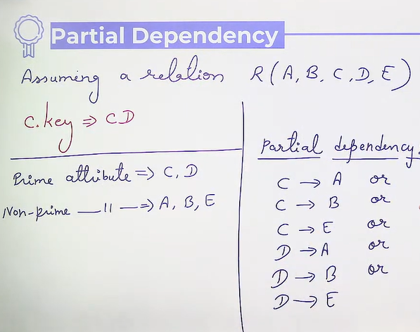
A relation R is said to be in 2NF if it is already in 1NF and there is no any non-prime attribute R which is partially dependent on prime attribute of R.
is present in FD, then it is not in 2NF.
Partial Dependency: Partial dependency in a relational database occurs when a nonprime attribute (i.e., not part of any candidate key) is functionally dependent on only a part of the candidate key, rather than the entire candidate key.
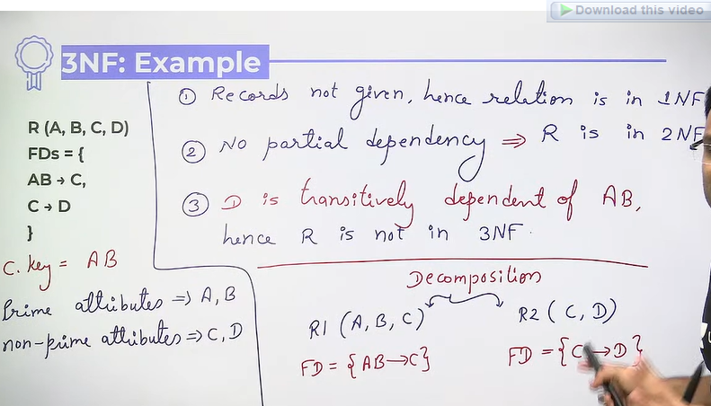
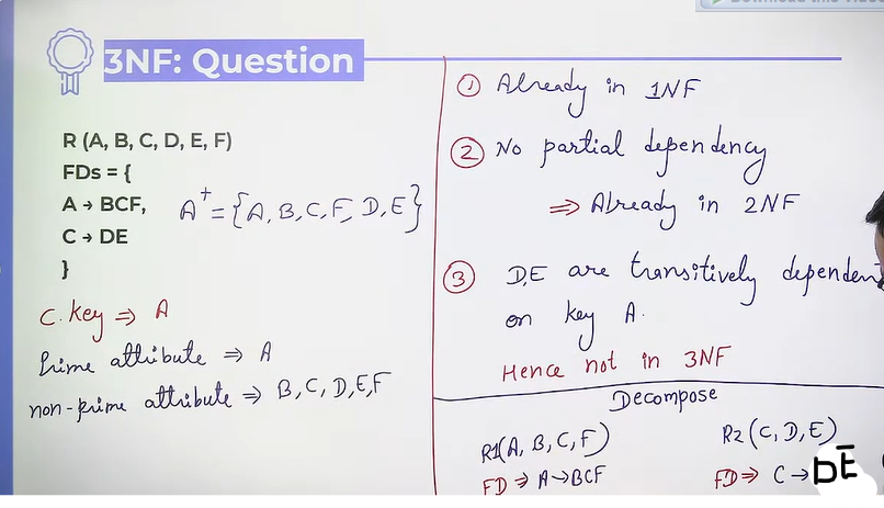
3 NF : 3rd Normal Form
A relation is said to be in 3NF if there is already in 2NF and there is no any non-prime attribute in R which is transitively dependent on the key of R.
It won’t be 3 NF if
- Not in 2NF
- Key → X, X → A or
NPA→NPA
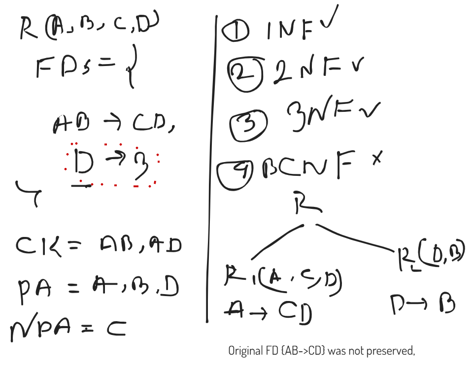
BCNF : Boyce Codd Normal From
A relation R is said to be in BCNF if it is already in 3NF and for every functional dependency A→B, A should be super key in R.
Lossy, Lossless, and Dependency Preserving Decomposition
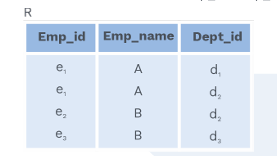
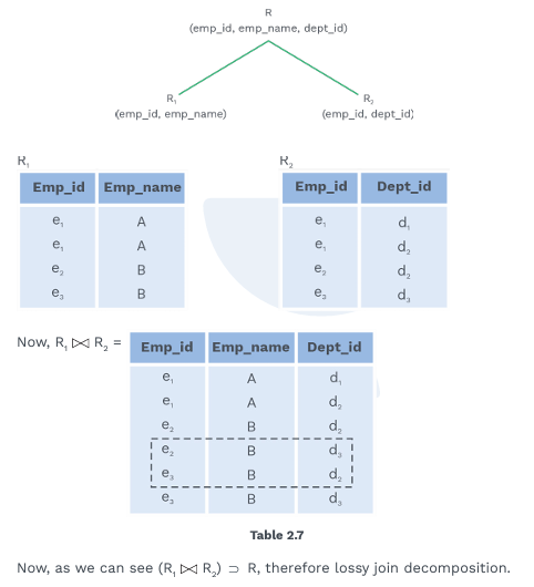
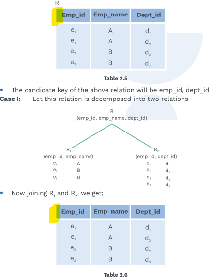
Lossy Decomposition: The decomposition of relation R into R1, R2, R3, R4 … RN is lossy when the join of R1, R2, R3…RN does not produce the same relation as in R.
Lossless Decomposition: The decomposition of relation R into R1, R2, .., Rn is lossless when the join of R1,R2,…,Rn produces the same relation as in R.
- Upto 3NF all decompositions are lossless and dependency preserving
- BCNF may give lossy decomposition and may/ mayn’t be dependency preserving
Note:
- During the normalization process BCNF gives lossy decomposition, then BCNF decomposition wont be applied. Because, we will decompose until it gives lossless decomposition.
- Any relation with 2 attributes is always into BCNF.
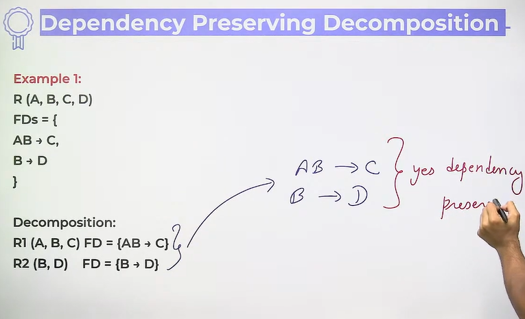
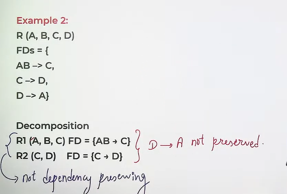
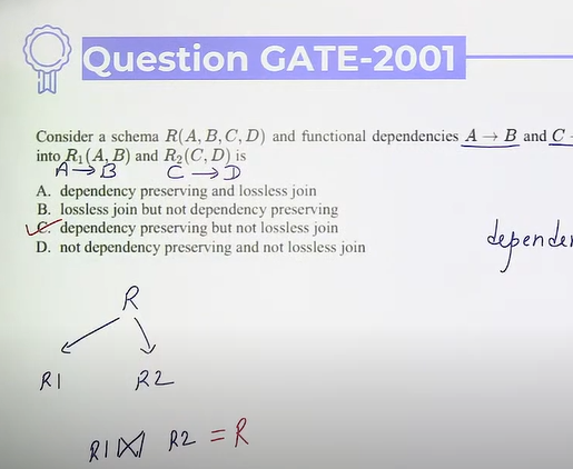
Dependency Preserving Decomposition: A decomposition D = {R1, R2, …, Rn} of R is dependency preserving with respect to a set F of functional dependency if
- Upto 3NF all decompositions are lossless and dependency preserving
- BCNF may give lossy decomposition and may/ may not be dependency preserving
SQL : Structured Query Language
Domain-specific language used in programming and designed for managing data held in RDBMS.
Operations
- Inserting
- Retrieving
- Updating
- Deleting and more
SQL Datatypes
- String
- Varchar
- Bit
- BOOL, BOOLEAN
- INT, INTEGER
- BIGINT
- FLOAT (size, d)
- FLOAT(p), p is 0-24, then it is float, if > 24, it will be in double.
More
- SQL is not case sensitivity
- Semicolon mandatory: nor always. If more than one sql statements to be run together, then semicolon is mandatory,
Select Command
Syntax: Select column1. column2 from table_name
To Select all columns: Select * from table
Using distinct: Select distinct column1, column2 from table [unique value of combination of column1, column2]
Where (Used to filter): select * from table where column2 = “something”
Sequence of running: from → where → select
Relational Operators in where:
- Equal =
- Not Equal <>
- Less than <
- Less than equal to <=
- Greater than >
- Greater than > =
Logical Operators
- AND : having multiple conditions
- OR :having multiple conditions
- NOT
Select * from order where NOT quantity > 10 = quantity ≤ 10
Between Operators: Used to filter records in the specific in range.
select * from table where quantity between 10 and 20. = 10 ≤ quantity ≤ 20
Return all such orders details when quantity is lesser than 10 or greater than 20 = select * from table where NOT between 10 and 20
Limit: Used to limit number of fetched records from a huge database table.
select * from table where price > 10 limit 10 = first 10 records where price > 10
show 4 records after leaving first 5 records = select * from table1 limit 5,4
NULL : null is a representation of having no value
select * from table where column is NULL
select * from table where column is not NULL
Aggregate Function: performs a calculation on multiple values and return a single value
- used in select
- it ignores null values
Min : select min(column) from table
Max : select max(column) from table
Sum : select sum(column) from table
Count : select count(column) from table ⇒ count the number of rows
Average: select avg(column) from table
In Operator: it allows you to specify multiple values in a where clause. it is shorthand for multiple or conditions.
select * from table where country in (”BD”, “USA”, “UK”)
Alias: used to give a temporary name to a table or column in a table
- used to make table names or column name more reliable
- only exists for the duration of the query
- created with the keyword : AS
Alias of table: select * from table1 as tb1
select * from table1 as tb1 inner join table2 as tb2 on tb1.column=tb2.column
Alias of column: select column1 as col1 from table where col1 = “Test”
select column1 as [Column One] from table
SQL Joins
Needed to retrieve records from more than one table
Requirement of Joint : 2 tables must have one common column
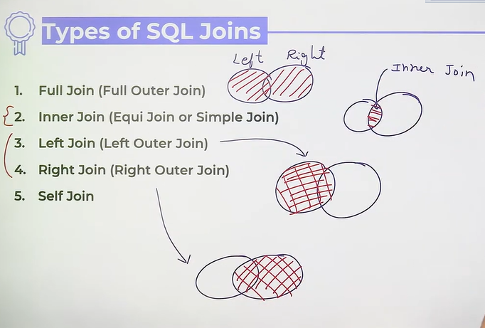
Types of Joins
Natural Join: Inner, Left and Right join
Inner Join
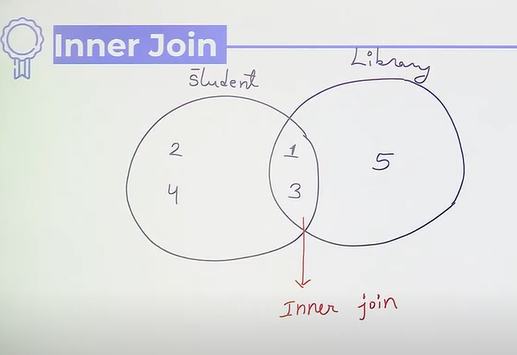
- select * from table1 inner join table2 on table1.column = table2.column
- without join: select * from table1, table2 where table1.column = table2.column
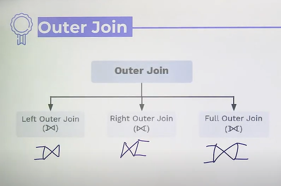
Left Join/Left outer join
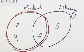
- select * from table1 left join table2 on table1.column=table2.column
- if there is no value of right table, then they will be filled with NULL
Right Join/Right Outer Join
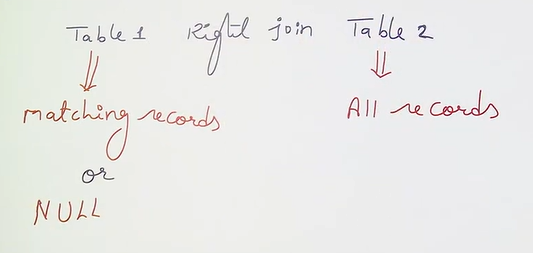
- select * from table1 right join table2 on table1.column = table2.column
Full Join/Full Outer Join
- all records from left and right table are fetched
- if any of them is not matching, then records are filed NULL
- select * from table1 full join table2 on table1.column = table2.column
Self Join
- only one table is involved, act like inner join
- select * from table1 as tb1, table2 as tb2 where tb1.column=tb2.column
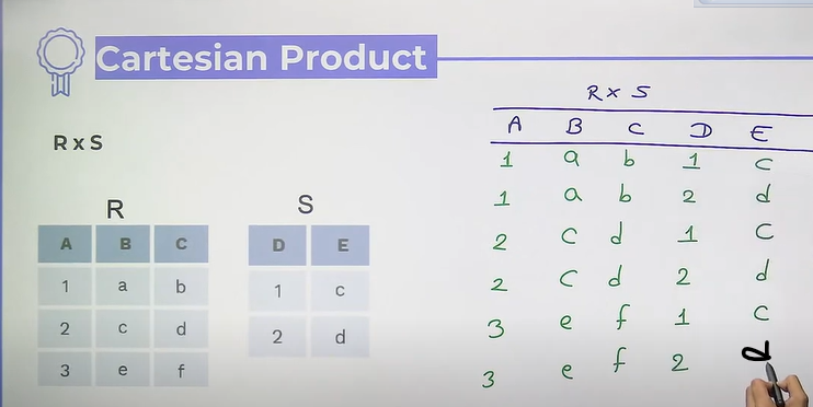
Cartesian Product
- super set of all combinations of all records
- no any common column is needed
- select * from table1, table2
- if table 1 has c1 column and r1 rows, table2 c2 and r2
then cartesian product : column = c1 + c2, rows = r1*r2
Group By clause
- SELECT count(customer) as [Total Customer], status as [Status] from shippings group by status

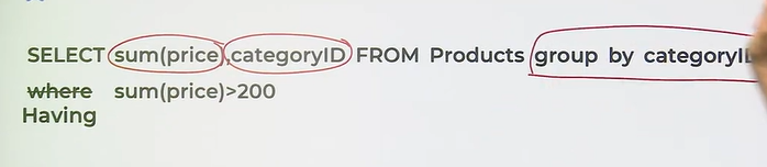
select sum(price), catID from products where group by catID
- select sum(price), catID where catID > 2 group by catID
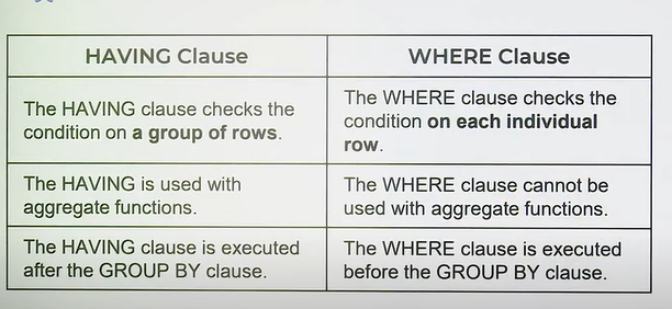
WHERE should be used before executing the group by

Can’t use where after group by/with aggregate function. HAVING
Having Clause
The having clause in sql is used if we need to filter the result based on aggregate functions such min, max, sum, avg, or sum. The having clause was introduced because the where clause does not support aggregate function. Also, group by must be use before the having clause.
Execution: where → group → having
Set Operators
- Used to combine results from two or more select statements
- Syntax : (select * from table1) SetOperation (Select * from table2)
- no. of columns selected by both queries must be equal
Types
- Union
- duplicate rows are eliminated
- Syntax : (select * from table1) union (Select * from table2)
- Union all
- it selects all rows from both select statements
- does not eliminate duplicates
- Syntax : (select * from table1) union all (Select * from table2)
- Intersect
- selects only common rows from both select statements
- Syntax : (select * from table1) intersect (Select * from table2)
- Minus/except
- it selects only those rows which are unique in first select statement
- Syntax : (select * from table1) except (Select * from table2)
ORDER BY Clause
- used to sort the result-set in ascending or descending order
- Ascending: SELECT * FROM table ORDER BY column1 asc
- Descending: SELECT * FROM table ORDER BY column DESC
- Default → Ascending : SELECT * FROM table ORDER BY column1
- it executes at last
- Multiple column : select * from table order by column1 desc, column2 asc [if column1 is same for multiple rows, then column2 will be considered]
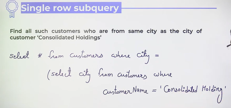
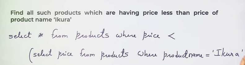
Subquery
A subquery or inner query or a nested query is a query within another sql query and embedded within the where clause.
Types of subquery
- Single row subquery : fetch only one row
- Multiple row subquery : subquery return multiple rows
Operator Used with
- In : used for equal to or not equal to comparison only
select * from table where in (sub query)
Find all customers, who are in supplier city.
select * from customers where country in (select country from suppliers group by country)
Find all customers, who are not in supplier city.
select * from customers where country not in (select country from suppliers group by country)
Find all customers, who have placed more than 2 orders.
select * from customers where customer_id in (select customer_id from orders group by customer_id having count(order_id) > 2)
- any : can be used more operators
select column from table1 where column operator any (select column from table2 where condition)
Operator : =, <>, >, ≥, <, ≤
Find the productName of all those products which have their orders quantity larger than 50.
select prodductName from products where productID = ANY (select productID from orders where quantity > 50)
Find the productName of all those products which having productIDs less than any of the product having orders Quantity equal to 1.
select productName from products where productId < any(select productId from orders where quantity=1)
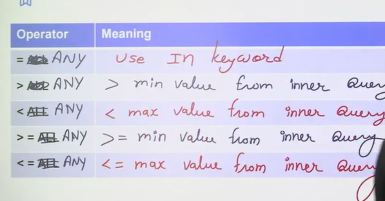
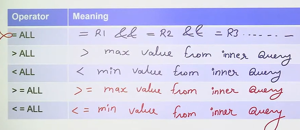
- all
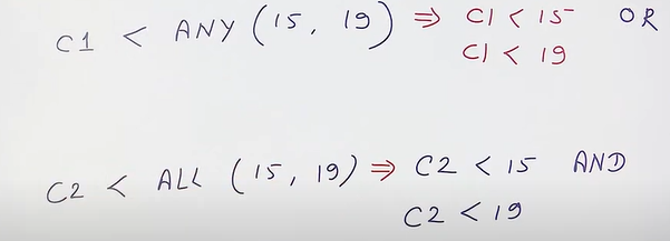
select column from table1 column operator all(subquery)
Select all products which have productId less than all of the id which have order quantity 1.
select * from products where productId < all(select producId from orders where quantity = 1)
Finds all employees whose salaries are greater than the salary of all the employees in the Sales department with departmentID 2.
select * from employee where salary > all(select salary from employee where departmentID = 2)
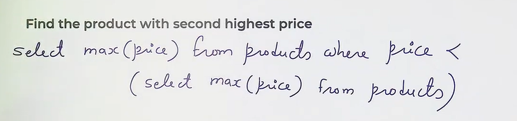
select * from employee where salary > (select max(salary) from employee where departmentID = 2)
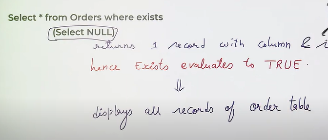
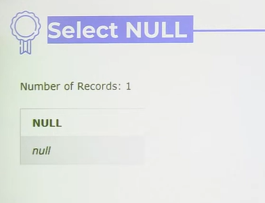
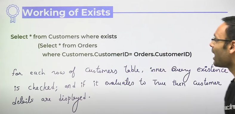
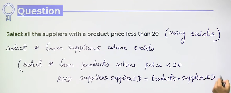
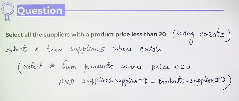
- exists :
- used to test for the existence of any record in a subquery
- returns true if the subquery returns one or more records
- work for multiple and single row subquery
select * from where exists (subquery)
- In : used for equal to or not equal to comparison only
- NOT Exists : Opposite of exists
Why subquery not join ?
- readable and understandable
- better performance
- joins may have redundant data
Other wise join performs better than subquery.
Relational Algebra
Relational algebra is a procedural query language, which takes instance of relations as input and yields instance of relations as output.
The main application of relational algebra is to provide a theoretical foundation for relational databases, particularly for query language.
Basic Operators
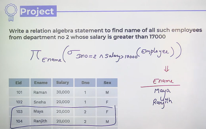
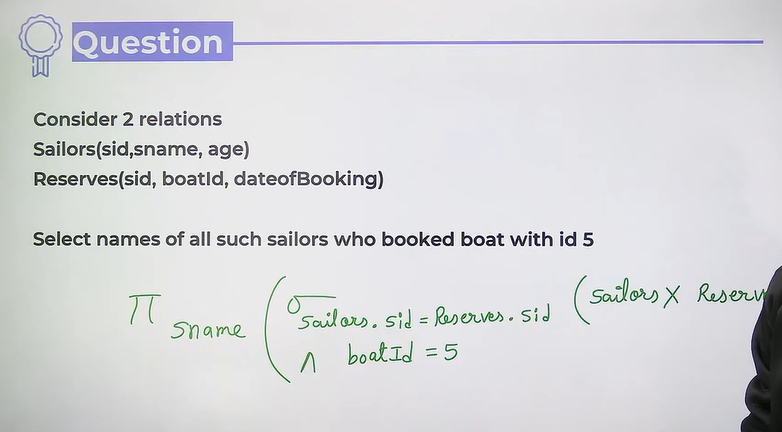
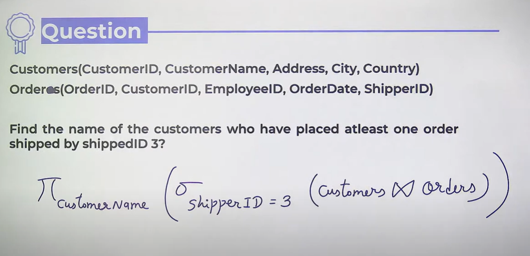
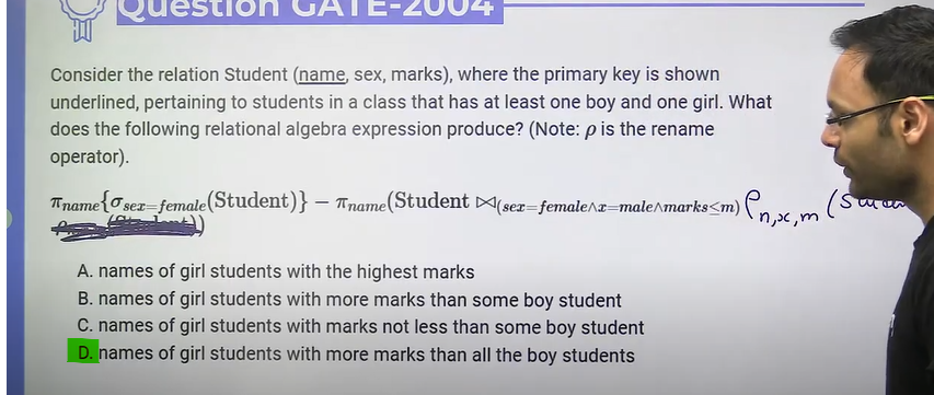
- Select : Same as SQL Select * from where condition
→ and, → OR
- Project : Selecting specific columns, similar to select distinct col from, projects should be written in outermost
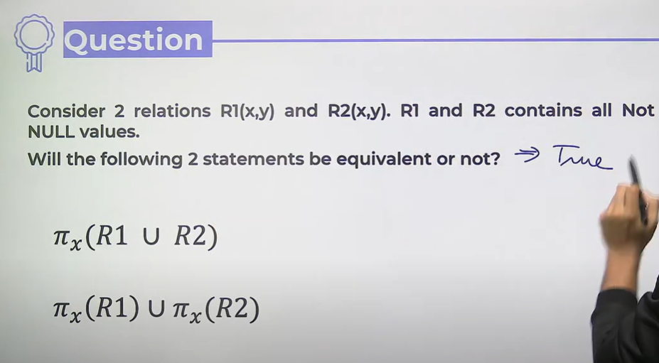
- Union
- no column of should be same, consecutive column of each table type must be same, duplicates are eliminated
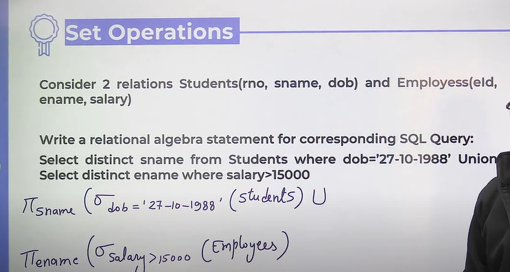
- no column of should be same, consecutive column of each table type must be same, duplicates are eliminated
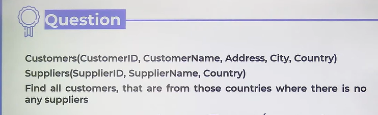
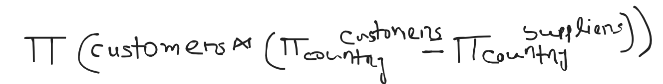
- Set difference
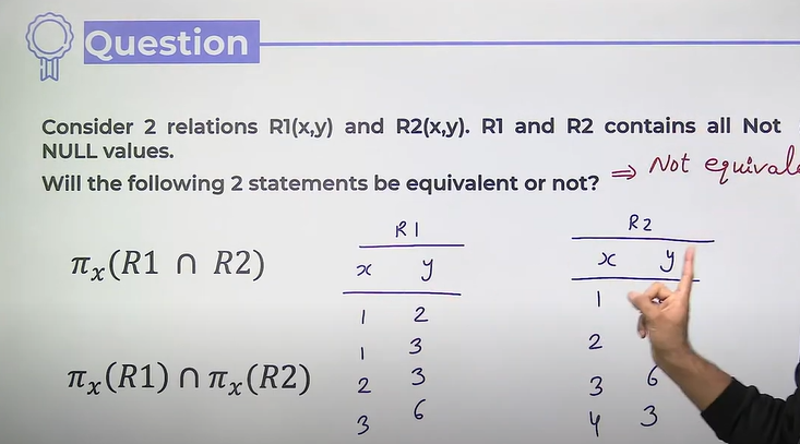
- Intersection
- Cartesian Product
- Joins
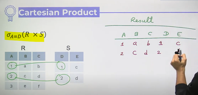
- Condition Join : join with conditions
- Equi Join : if condition is only equal to
- Natural Join: requirement is both relations should have at least one column name common and they matched automatically
- Condition Join : join with conditions
- Rename : as aliasing in SQL
⇒ Students renamed as s (table name)
⇒ Giving new name to column and table
⇒ Just columns are re named not the table
⇒ RollNo column named as R
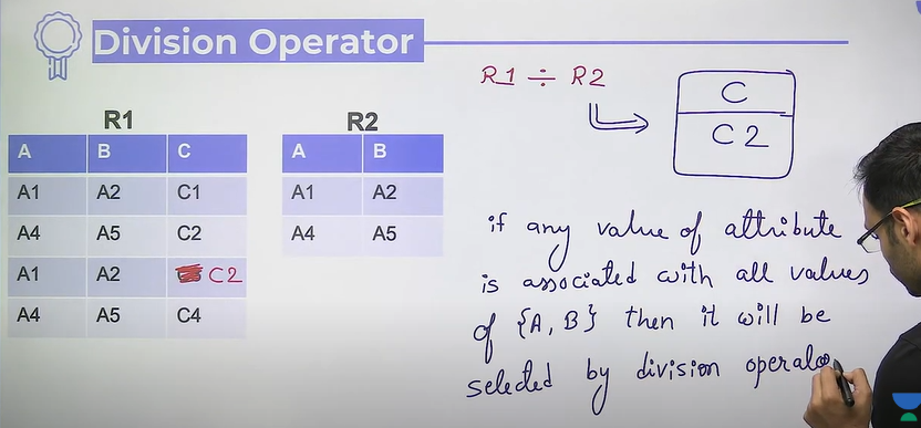
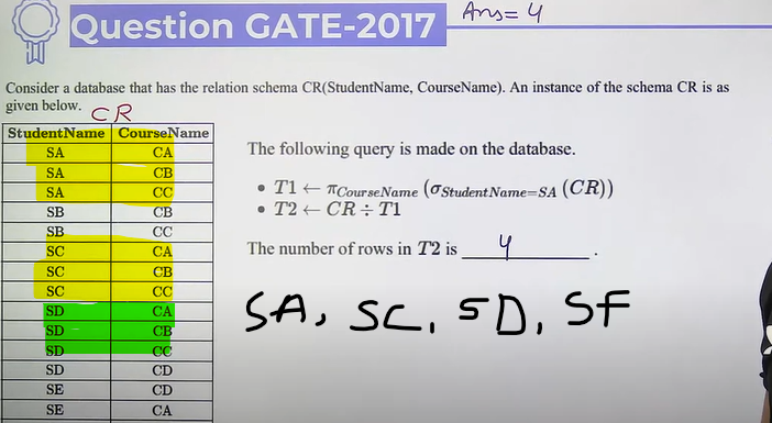
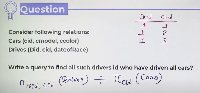
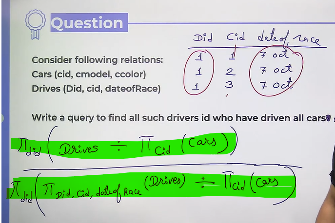
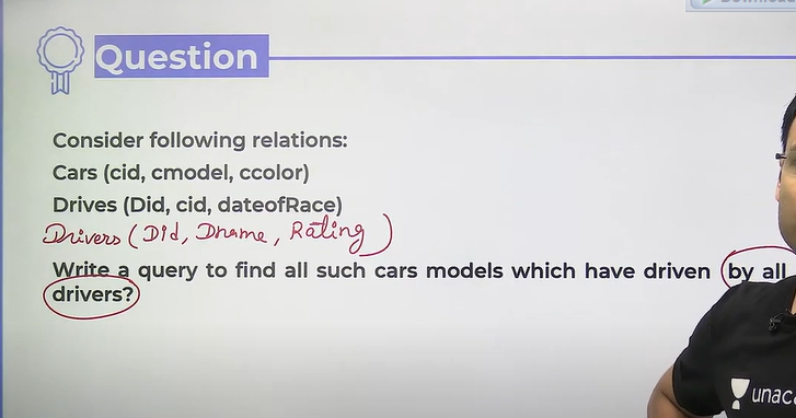
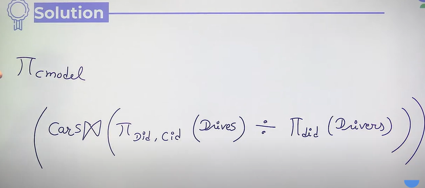
- Division
-
Attribute set of R2 should be a subset of R1
- Answer will be that value of R1 which is associated with all the rows of R2.
- used in for all case
-
Transaction
Logic unit of database which includes one or more database access operations.
Commit
Rollback: Back to last commit
ACID Property of Transaction
- Atomicity: All or none
- Consistency: All transaction should provide consistent result.
- Isolation: If multiple transaction which are running on same database produce the result in such a way that all are running in isolation.
- Durability:
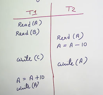
Schedule
Collection of multiple transactions running on same database.
Concurrency:
Why Concurrency
- Improved throughput
- Resource utilization
- Reduced waiting time
Problem with concurrency
- Recoverability problems
- Deadlock
- Serializability issues
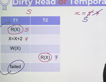
- Dirty read or temporary update problem
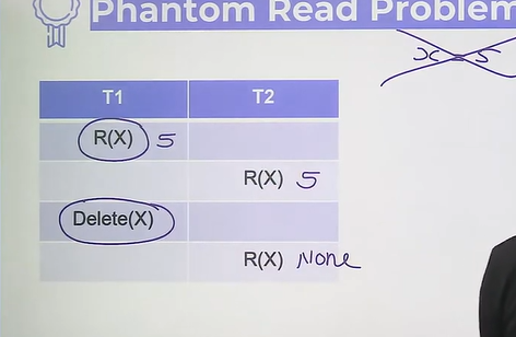
- Phantom read problem
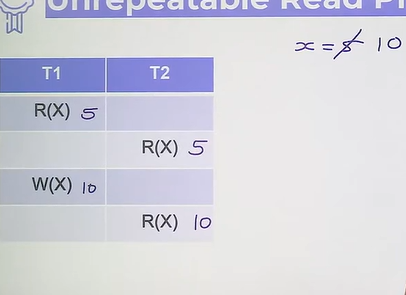
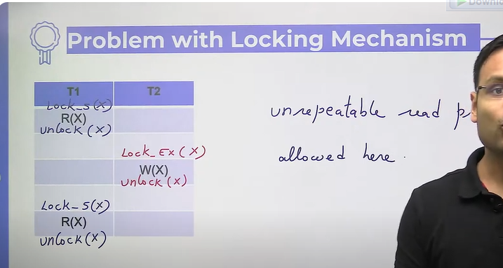
- Unrepeatable read problem
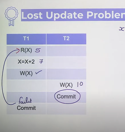
- Lost update problem
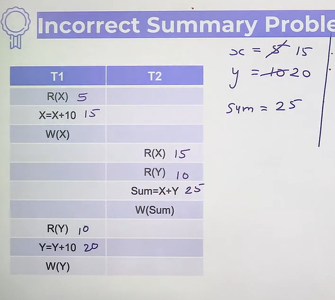
- Incorrect summary problem
Good vs Bad Schedule
Good schedule: concurrent schedules which provides consistent result.
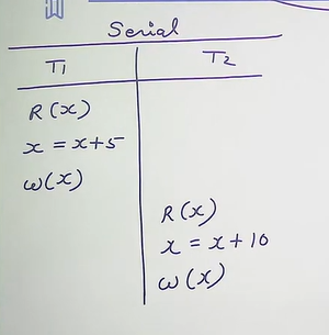
Serial vs Non-serial Schedule
Non-serial: concurrent
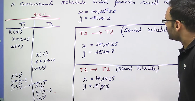
Serializable Schedule: A concurrent schedule which provides result as a serial schedule.
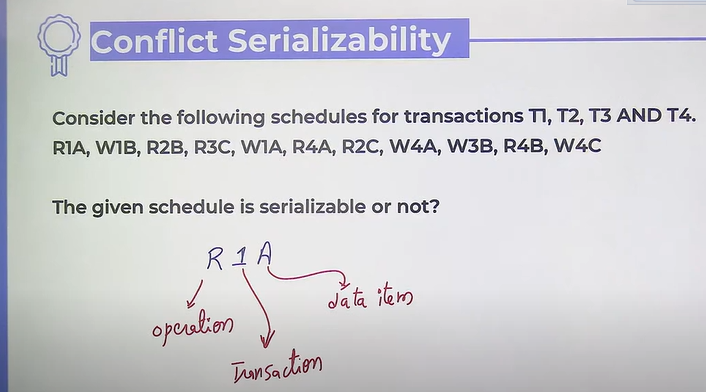
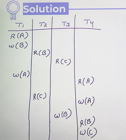
Checking Serializability
- Conflict Serializability
- 2 databases statements are conflicting if and only if
- both are in different transactions
- both are accessing the same data item
- at least one of them is write operation
- Read-read no conflict
- Conflict Equivalent
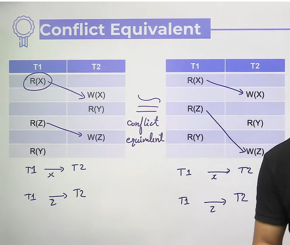
- Conflict Serializability
- Given a concurrent schedule S, find a serial schedule S’, such that
S conflict equivalent S’
S is a conflict serializable.
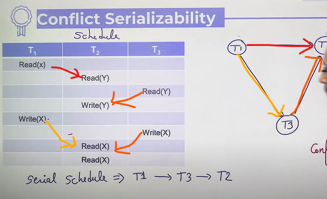
- To prove a given schedule conflict serializable we will use a graph ⇒ conflict precedence graph (Directed graph)
- Vertices ⇒ Transactions
- Edges ⇒ Conflicts
- If conflict graph has a cycle, then it is not conflict serializable
- Given a concurrent schedule S, find a serial schedule S’, such that
- 2 databases statements are conflicting if and only if
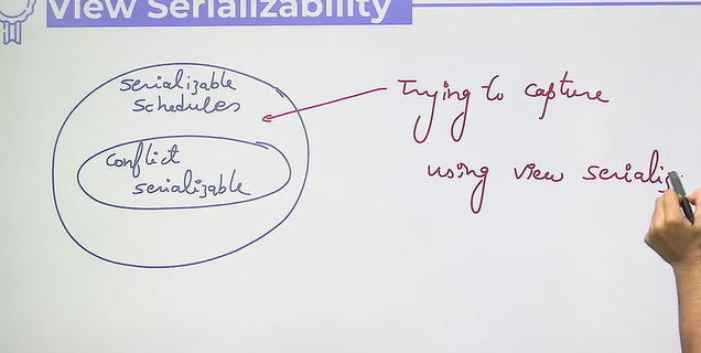
- View Serializability
- because of conflict serializability has too hard rules
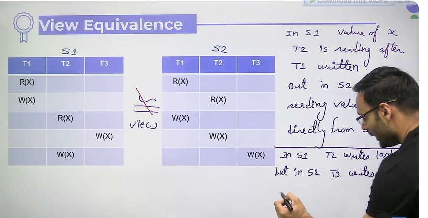
- 3 points to remember: for every datwa item
- who reads from database
- who reads from others written value
- who writes last
- View equivalence
- S1 and S2 are view equivalence if both are following similar sequence rules of view serializable
- View Serializability
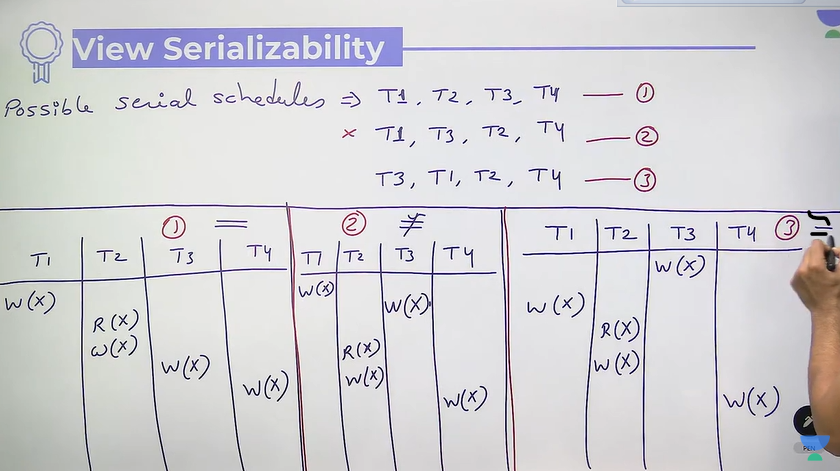
- A schedule is called view serializable if it is view equivalent to any serial schedule
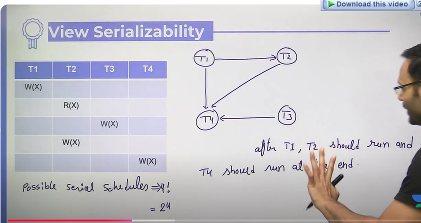
- If there is a concurrent schedule S, and it is serializable iff
S view equivalence S’, where S’ is any serial schedule
- Will make a graph based on rule 2 and 3
- who writes last will be in last in the sequence

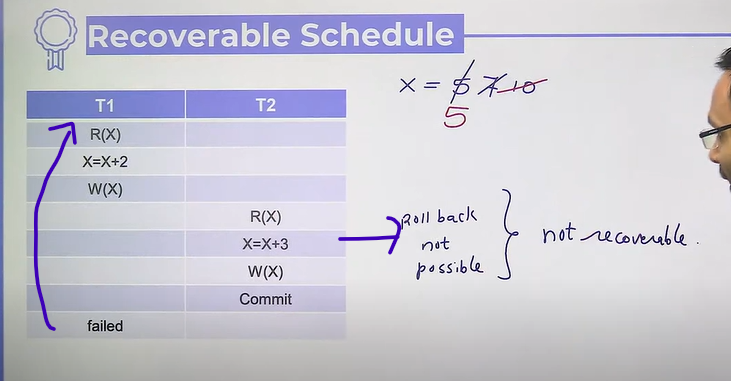
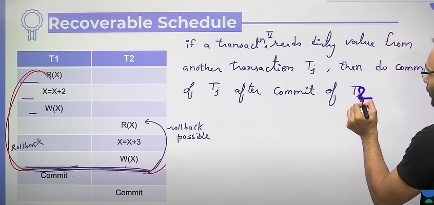
Recoverable Schedule
When no any committed transaction should be rolled back.
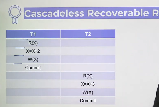
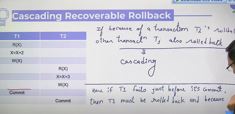
- Cascadeless recoverable rollback
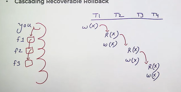
- Cascading recoverable rollback
Serializability is not possible in practically. Practical ⇒ Locking protocols…
Locking Protocols
What is Lock?
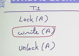
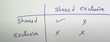
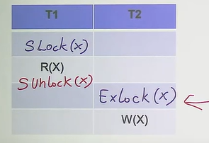
Types
- Shared : Taken for read, so that multiple read can be allowed
- Exclusive : taken for write
Busy waiting
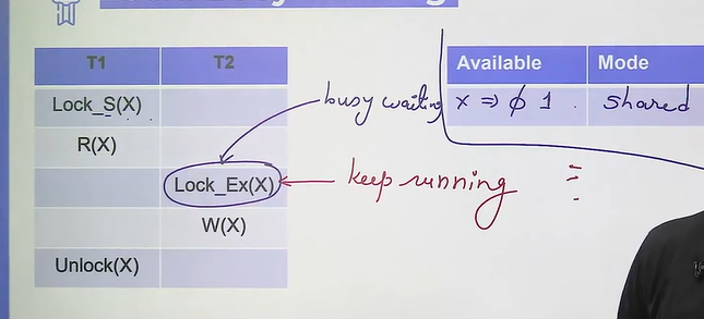
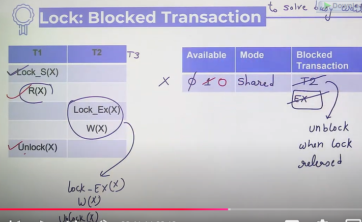
Block transaction
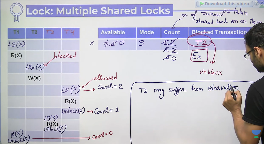
Multiple shared Lock ( with Starvation)
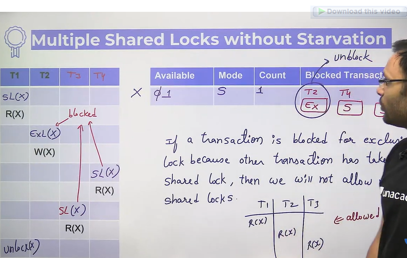
Multiple shared Lock without starvation
Problem With Locking mechanism
2 Phase Locking Protocol
1 Phase : Locking
2 Phase : Unlocking
Basic 2 phase locking protocols (2PL)
- Systematic locking mechanism
- Once unlock done, a transaction is not allowed to lock any database item
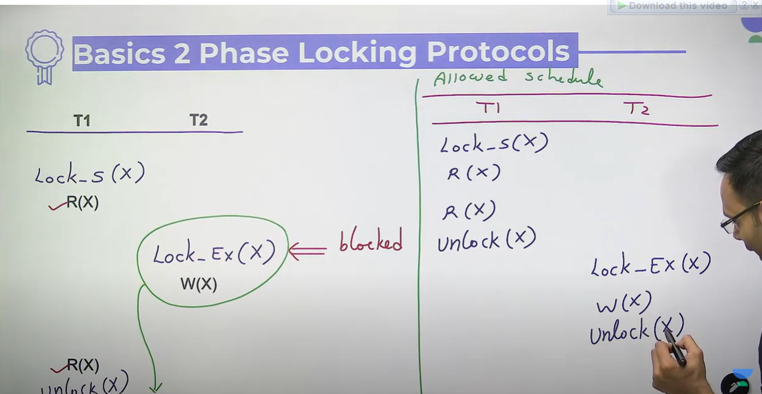
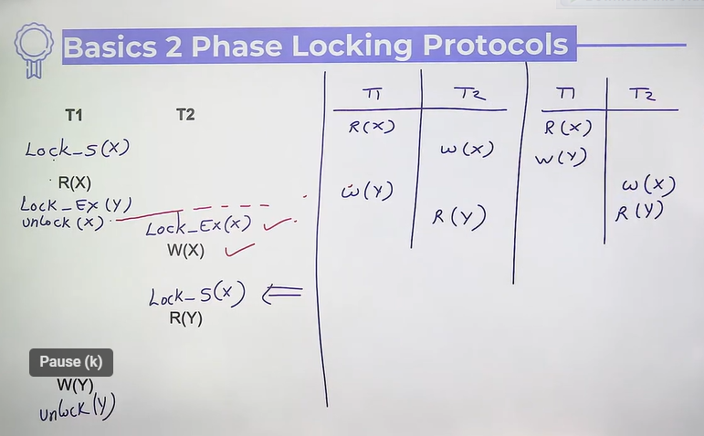
- Every schedule which is allowed under basic 2PL, is conflict serializable also.
- 2 PL
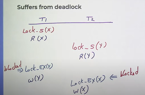
- Suffers from starvation
- suffers from deadlock
Database Record Storage
File System
Logical block
Indexing
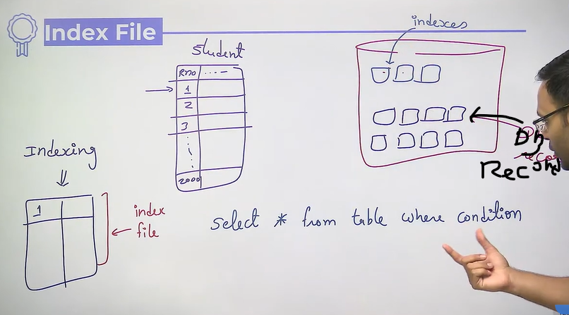
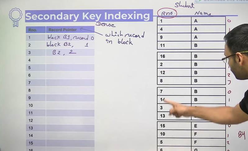
Dense vs Sparse Index
Dense: index record is for each database record
Sparse: index record is for a few database record only
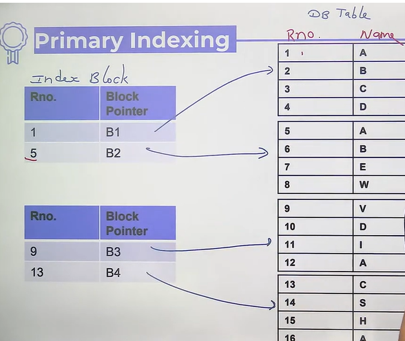
Indexing Techniques
- primary
- indexing done on primary key or any super key
- data must be ordered on index
- its always sparse index
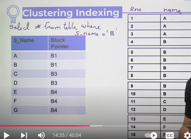
- clustering
- indexing done non-key field
- data must be ordered on index field
- It is sparse → indexing is done for each unique non-key
- secondary-key
- indexing done on primary key or any super key
- data must not be ordered on index field
- it can be dense or sparse
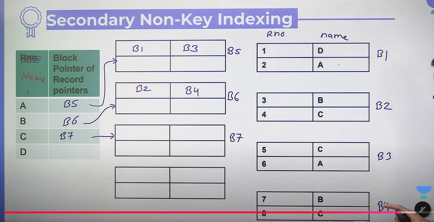
- secondary non-key
- indexing done on non-key field
- data must not be ordered on index field
Was Linear searching..
B Trees
- Tree based indexing
- dynamic indexing technique
- based on insertion and deletion, the tree automatically adjusted
- self balancing search tree
- it grows horizontally and vertically
An order-p B-tree
- maximum children p
- every node other root should have atleast keys and ceil p/2 child
- in every node there are at most (p-1) keys and p tree pointer
- root can have minimum 1 keys and 2 tree pointer
- all leaves appear on the same level
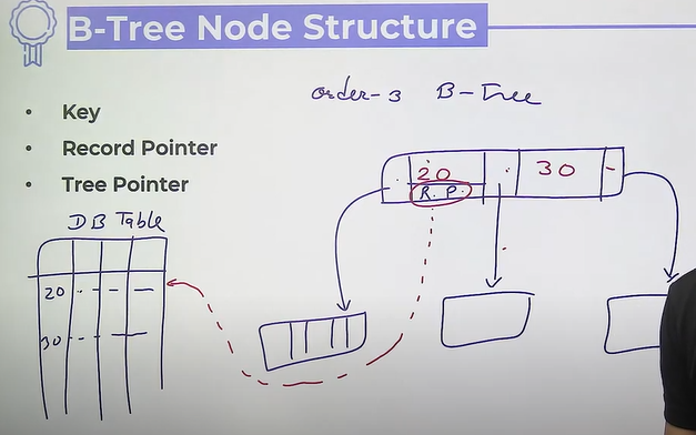
Node structure
- key
- record pointer
- tree pointer
P-order B-tree
Total nodes = n