Communication Engineering
| Created by | Borhan |
|---|---|
| Last edited time | |
| Tag | Year 3 Term 1 |
Resources
- Ma’am’s slide.
- Bangla :
https://www.youtube.com/watch?v=AJ-QfSSgXTg&list=PLMjaJoGgWV1nNjZXvcps2TrjdloXQxwbn&index=1&ab_channel=RojibEEEAcademy (Recommended if you are following ma’am slide.)
- Superheterodyne Receive: [90,93]
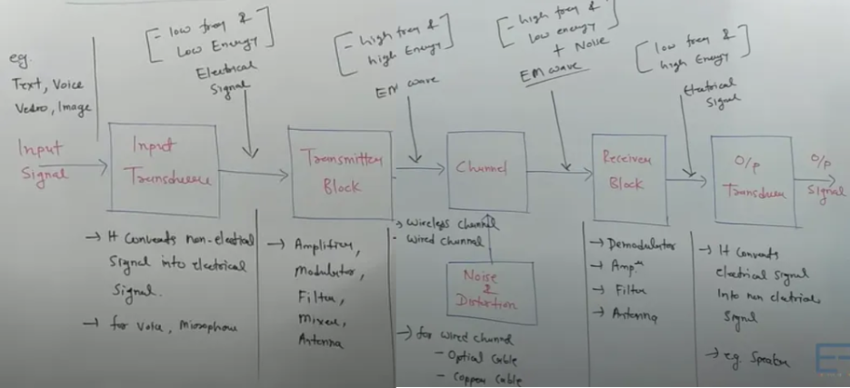
Communication System
Classification of Electric Communication System
- Unidirectional system or simplex system
- Bidirectional system or duplex system
- Half duplex system
- Full duplex system
| Basis for Comparison | Simplex | Half Duplex | Full Duplex |
|---|---|---|---|
| Direction of Communication | Unidirectional | Two-directional, one at a time | Two-directional, simultaneously |
| Send / Receive | The sender can only send data | The sender can send and receive data, but one a time | The sender can send and receive data simultaneously |
| Performance | Worst performing mode of transmission | Better than Simplex | Best performing mode of transmission |
| Example | Keyboard and monitor | Walkie-talkie | Telephone |
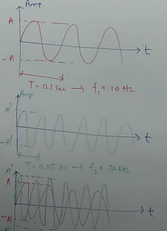
Time Domain Signal
- It is a plot of amplitude wrt time
- multiple signals make complex
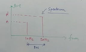
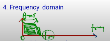
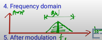
Frequency Domain Signal
- wrt frequency
- complexity is very less
Advantages
- Filtering
- Less complexity
- Stability
- Convolution of two signal = multiplication in frequency domain
Modulation
It is a process of modification of carrier signal wrt modulating (message) signal.
Carrier signal can be defined as a high frequency signal that is modulated by the modulating or the information signal.
Need of Modulation
- Height of antenna : reduction of size in antenna
,
Length of antenna,
dipole,
monopole,
small antenna,
We can increase to decrease the .
- Radiated power by antenna: , power increases when increases
- Multiplexing: FDM, TDM, CDMA
- High Bandwidth
- Narrow Banding signal
Classification of Modulation
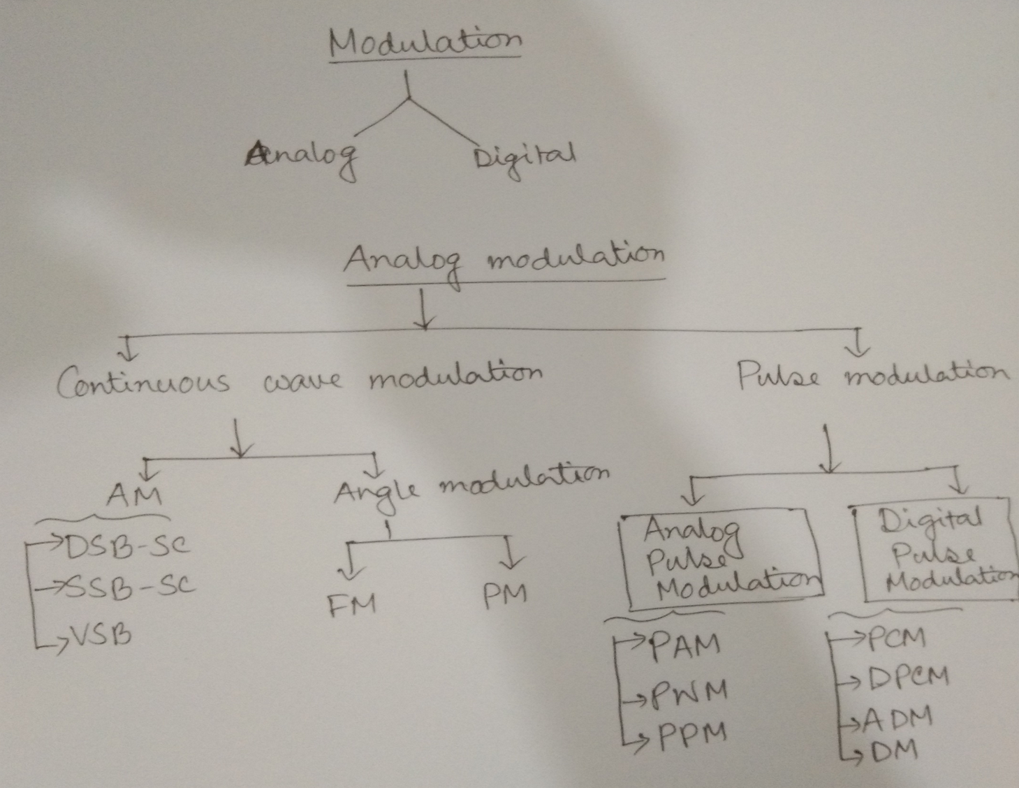
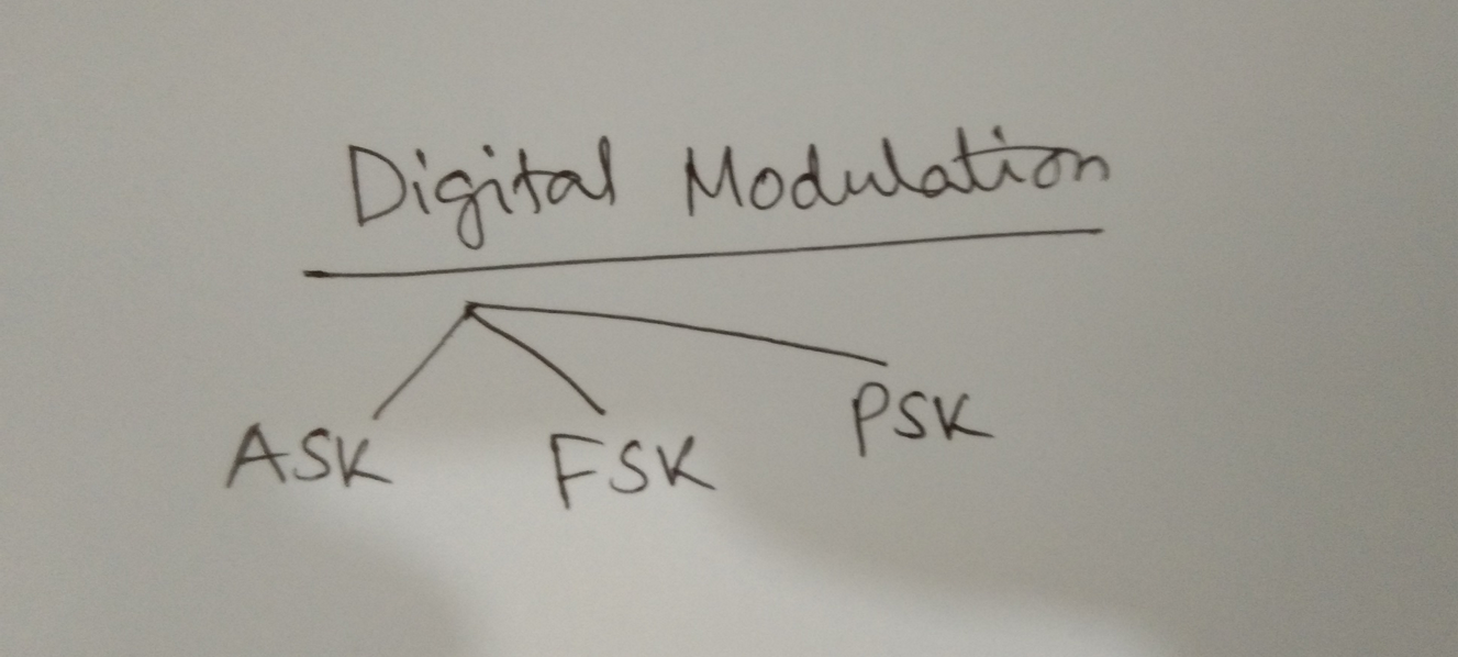
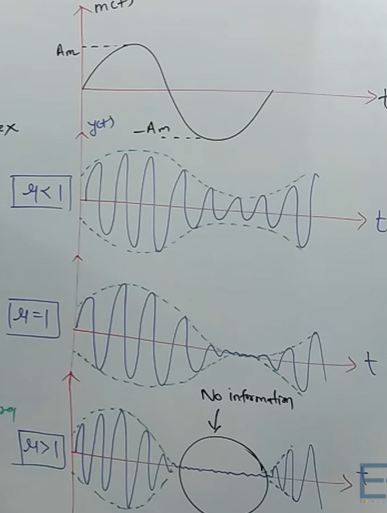
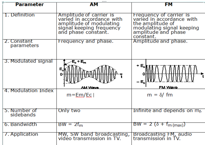
Amplitude Modulation
It is the process in Amplitude of carrier signal changes wrt message/ modulating/ information signal.
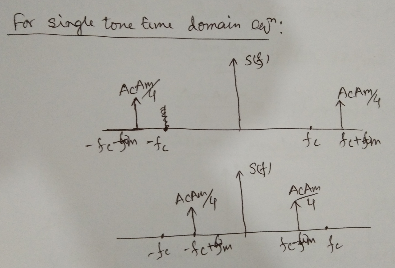
For single tone,
where, modulation index
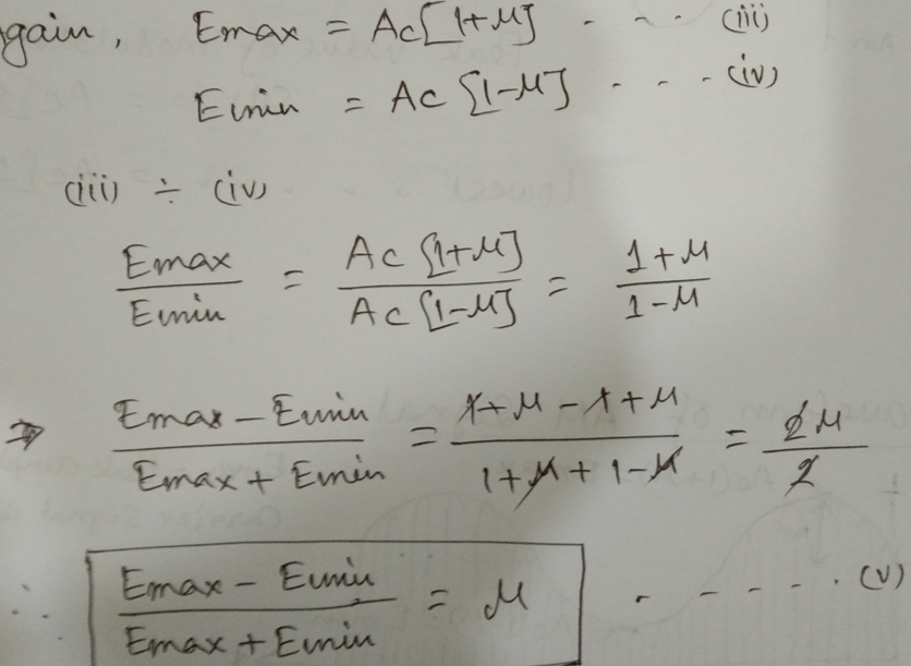
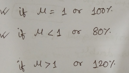
Modulating Index
AM Signal Transmitted power
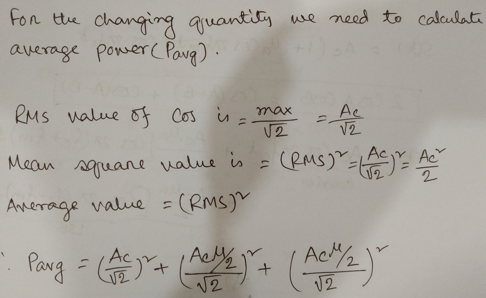
Total Transmitted Power,
Powe of carrier, , It is redundancy → it doesn’t have information
has information, it is called power of sideband.
Power of Upper Sideband,
Power of Lower Sideband,
Power of sideband,
Total Power,
Efficiency of AM Signal
It is based on . Because, it has information.
Redundancy
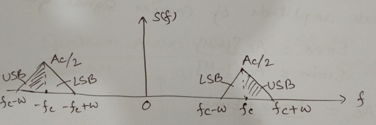
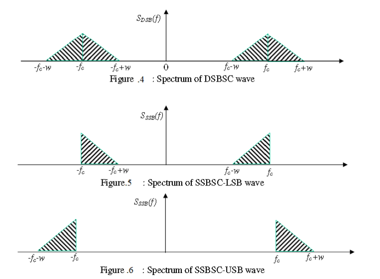
DSB-SC : Double Side Band Suppressed Carrier
Transmission in which frequencies produced by amplitude modulation are symmetrically spaced above and below the carrier frequency and the carrier level is reduced to the lowest practical level, ideally completely suppressed.
- We don’t send carrier signal
- Only LSB and USB are there
- It has 180 degree phase reversal at zero lossy of modulating signal
Advantages
- Lower Power Consumption
Disadvantages
- Complex detection
Applications
- Analogue TV
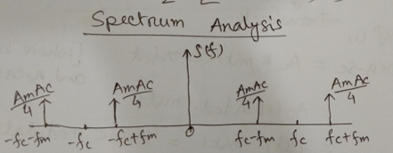
AM signal,
[, ]

Balance Modulator DSB-SC
- Consists of two identical AM modulation
- one input m(t)
- another input -m(t)
- The summer block is used to sum those
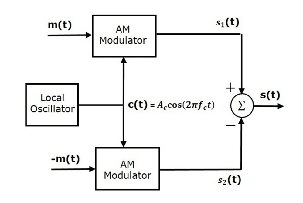
By comparing with the standard form of DSB-SC, we will get the scaling factor as
Ring Modulator DSB SCs
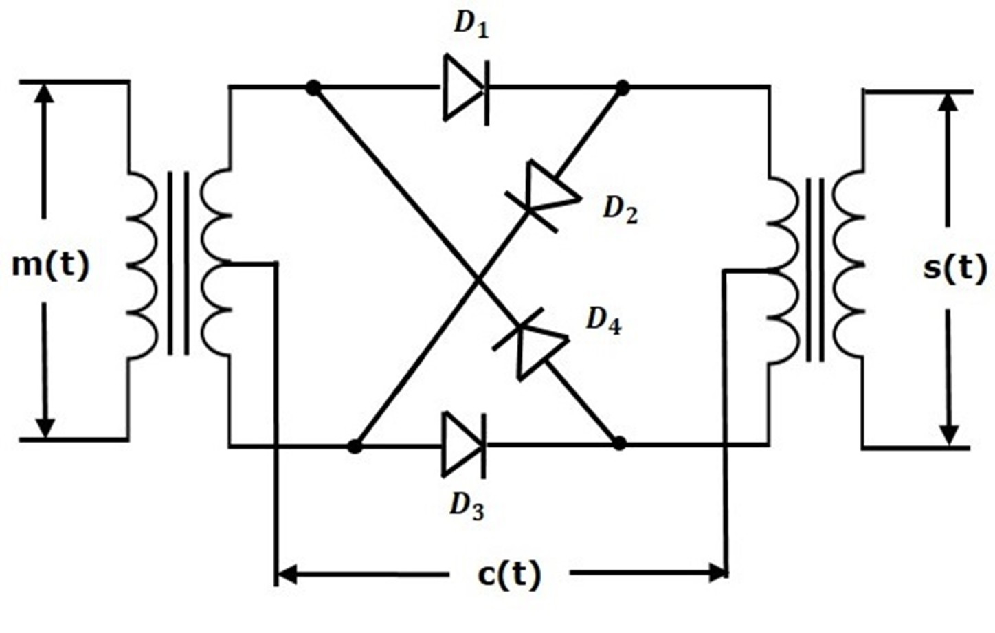
For Positive half cycle
- D1, D3 = on, D2, D4 = off
- message signal multiplied by +1
- are connected in ring structure
- Two center tapped transformers are used
- Carrier signal is applied between two transformer
- Carrier signal controls the diode
For Negative half cycle
- D2, D4 = on, D1, D3=off
- message signal multiplied by -1
We will get DSB SC wave s(t), which is just the product of the carrier signal c(t) and the message signal m(t), which represents DSB-SC wave and is obtained at the output transformer of the ring modulator.
SSB-SC : Single Sideband Suppressed Carrier
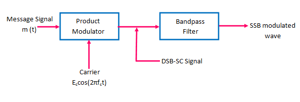
- Removes any of sideband along with carrier
- Bandwidth =
or,
We can use SSB-SC for Audio, Video signal but voice signal. Because of gap.
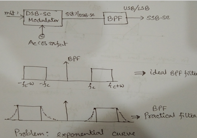
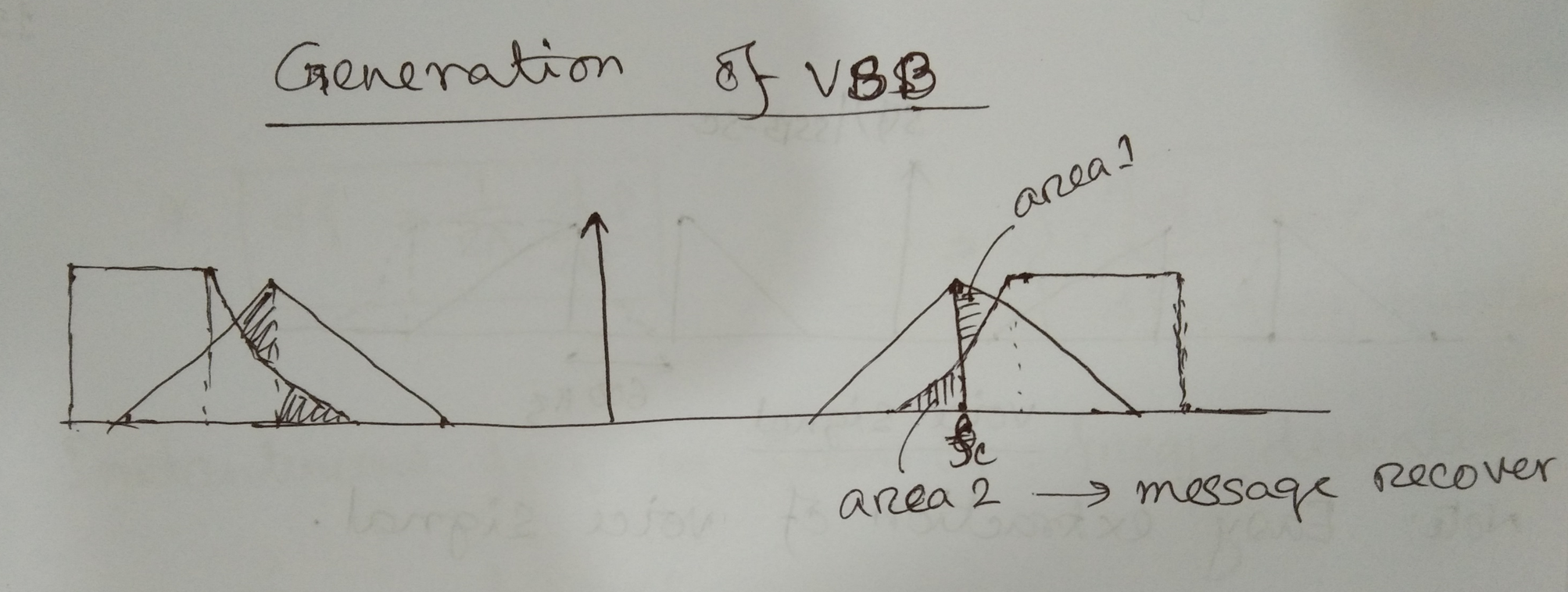
VSB : Vestigial Sideband Generator
- Used to transmit video signal
- Modify the BPF of SSB-SC
- Voice : 300 - 3500 Hz (SSB-SC)
- Audio Signal (20-2000 Hz)
- Video Signal (0-4.5 MHz) (VSB)
Demodulation of AM
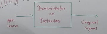
Envelope Detector
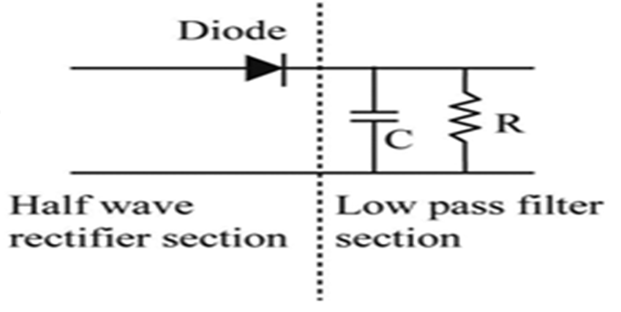
- It is a simple and highly effective system. This method is used in most of the commercial AM radio receivers
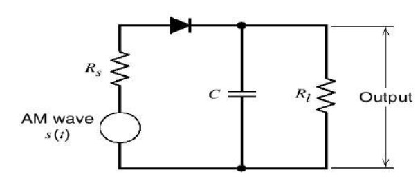
Positive Half Cycle
- Diode forward biased
- Capacitor charges rapidly
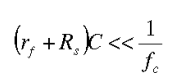
- Charge time constant (rf+Rs)C must be shorter than the carrier period
Negative/ Input signal falls
- Reverse
- Discharges through load resistor
- it continues until the positive next positive half cycle
- Discharging time constant must be long enough to ensure that the capacitor discharges slowly through between the positive peak of the carrier wave.
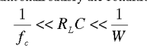
[W’ is bandwidth of the message signal]
Synchronous Detection
if , we should use this.
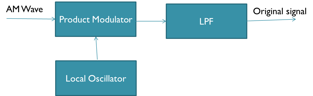
Local Oscillator
- generates carrier wave
- It is phase synchronous by Transmitter and Receiver
Advantages:
- Better quality than modulation
- less affected by noise
Draw Backs
- Transmitter and receiver are required
- More Complexity
Angle Modulation
Angle modulation is a modulation process in which the angle of the carrier wave or signal is changed with respect to the message signal or baseband signal.
Carrier Signal for Angle modulation,
Angle,
Amplitude,
Frequency, (in )
Phase =
⇒
⇒
⇒
⇒
…(i)
..(ii)
Carrier swing,
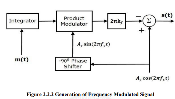
Frequency Modulation
Frequency Modulation (FM) is that form of angle modulation in which the instantaneous frequency is varied linearly with the baseband signal .
⇒ , Unit of
where
Expression
, we have to convert to frequency.
⇒
⇒
[]
[]
For single tone
Modulation index,
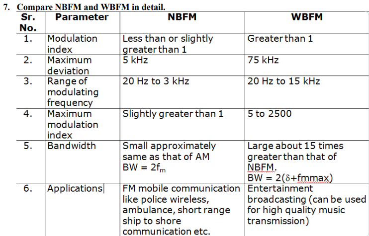
Types of FM:
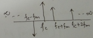
- Narrowband FM
This frequency modulation has a small bandwidth when compared to wideband FM. The modulation index β is small, i.e., less than 1. Its spectrum consists of the carrier, the upper sideband and the lower sideband. This is used in mobile communications such as police wireless, ambulances, taxicabs, etc.
⇒
where,
- Wideband FM
Ideal Bandwidth =
To get rid off this infinite bandwidth,
Carson’s Law :
- estimates the transmission bandwidth necessary for efficiently sending an FM signal without excessive bandwidth consumption
- Carson's rule states that the bandwidth required to transmit an angle modulated wave is twice the sum of the peak frequency deviation and highest modulating signal frequency.
- 90% power transmit
Phase Modulation
Phase modulation (PM) is a type of angle modulation where the phase of the carrier signal is varied in proportion to the the modulating signa .
⇒
where, = phase sensitivity of modulation =
Expression
For single tone,
Modulation index,
,
Phase derivation: Difference between phase of modulated carrier and phase of unmodulated carrier.
Unmodulated carrier =
Modulated carrier =
Single tone,
[]
Receivers
In radio communications, a radio receiver or receiver is an electronic device that receive radio waves and converts the information carried by them to a usable form.
- TRF : Tuned Radio Frequency
- SHR : Super Heterodyne Radio Receiver
Heterodyne Process
It is a process of mixing two signals having different frequencies in a non-linear manner to produce a signal with new frequency.
A special type of receiver that is used for this operation is caller Super heterodyne receiver (Superhet).
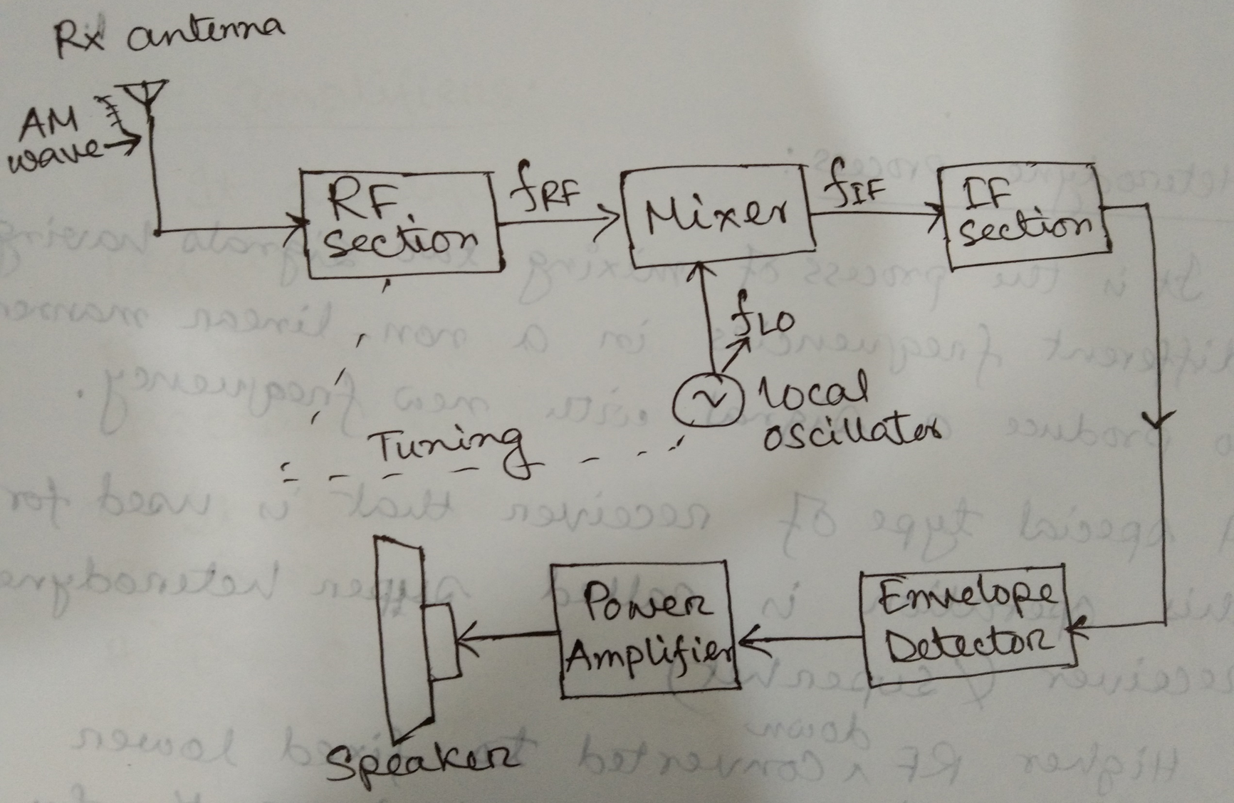
Superhet receiver sections
- RF Section
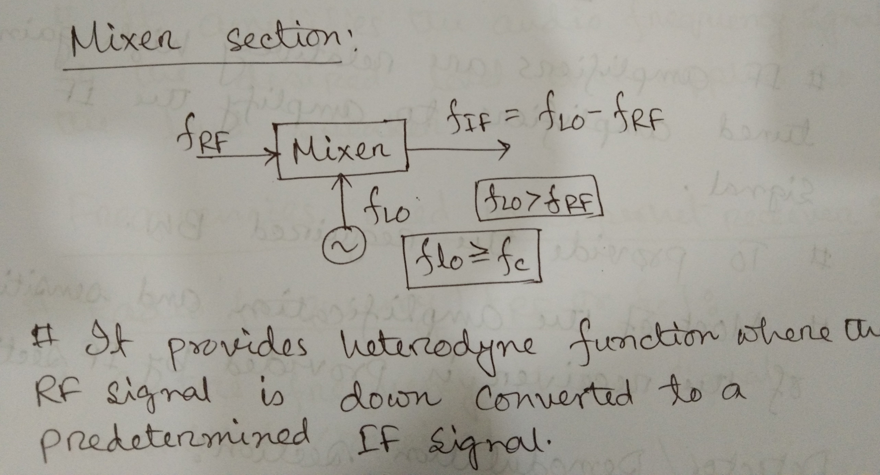
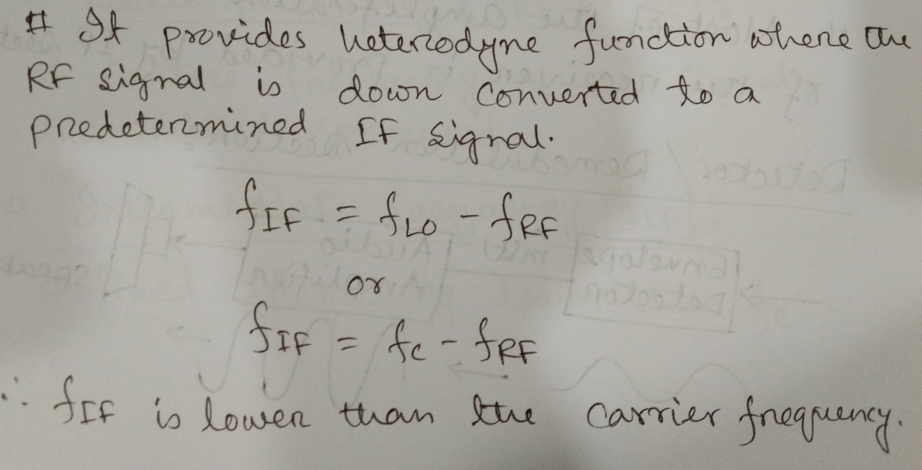
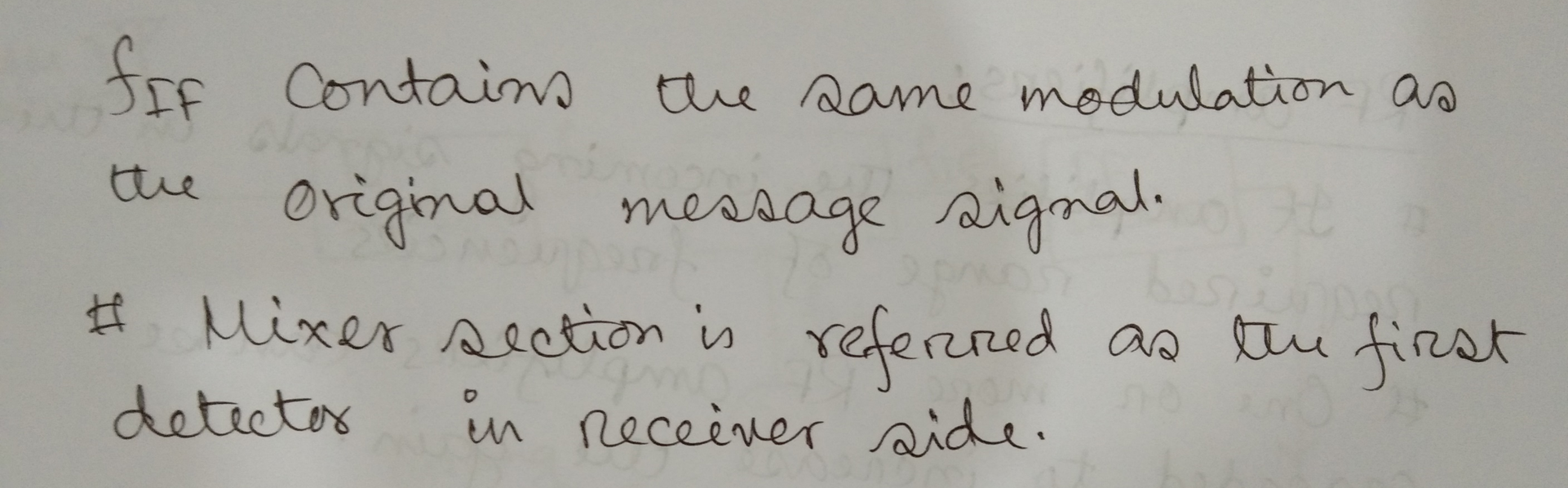
- Mixer Section/IF section
- Detector/Demodulator Section
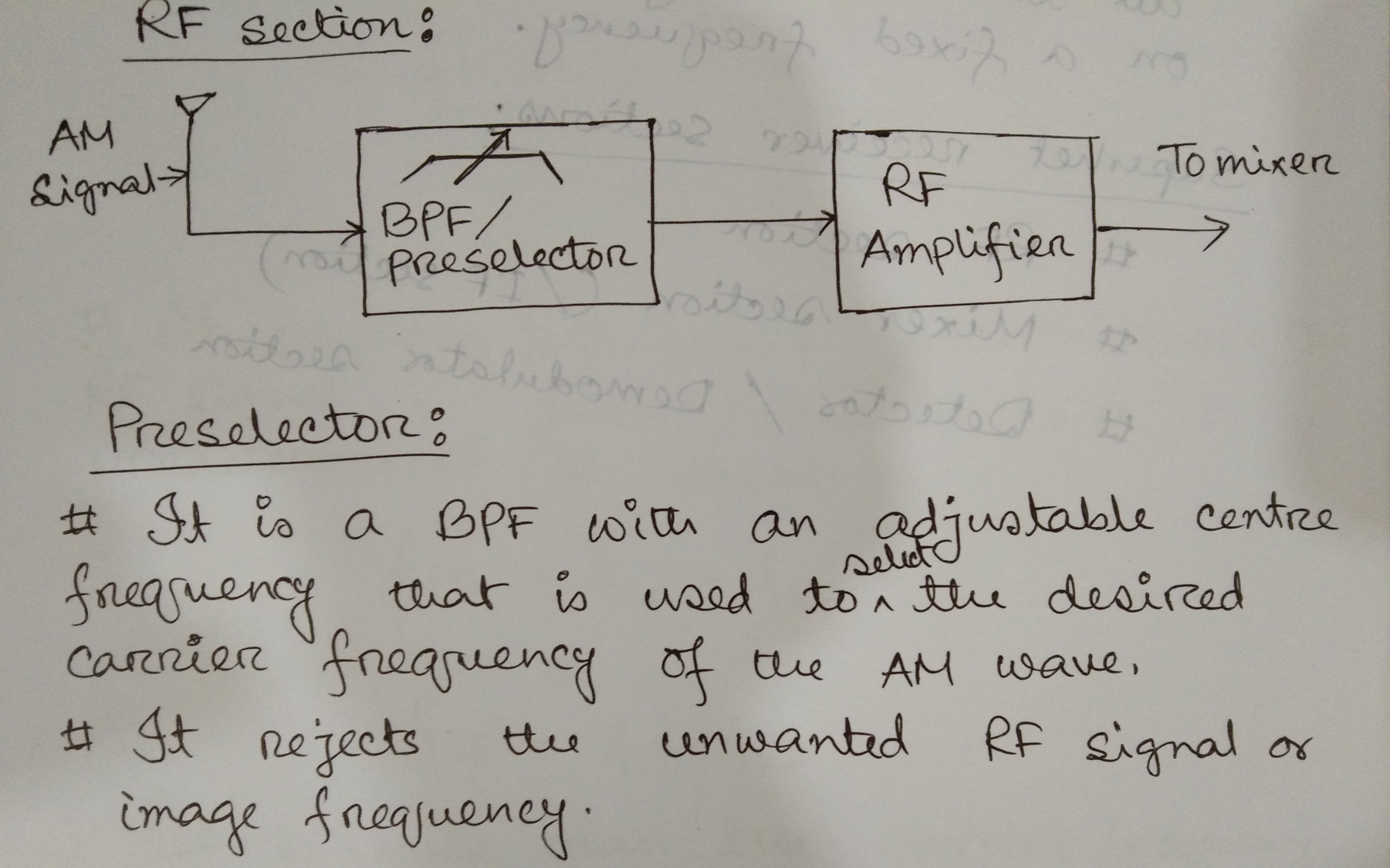
Preselector
- used to select the desire carrier frequency of AM wave
- It rejects unwanted RF signal or image frequency
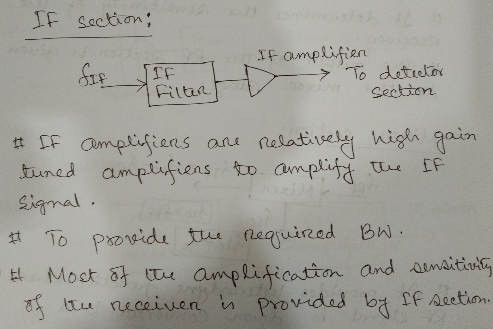
RF Amplifiers
- It amplifies the incoming signals in the required range of frequencies.
- One or more RF amplifiers can be cascaded to increase the gain.
- It determines the sensitivity of the receiver
- The output of the RF section is given to the mixer stage
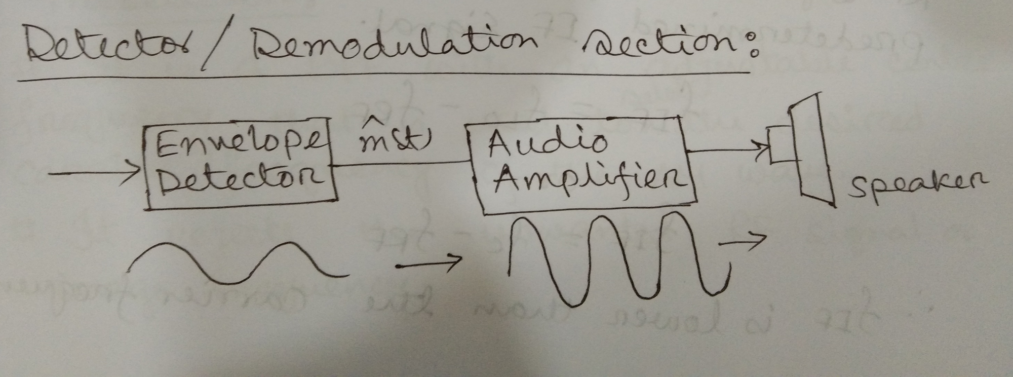
Envelope Detector
- Detector recovers the original information of the baseband signal from the output of IF amplifier
- The output of detector is low power audio signal
Audio Amplifier
- It amplifies the audio frequency signal to the desired level and applies to the loud speaker
Frequency used in Superhet receiver
- Radio Frequency : Centre frequency of the signal transmitted/received.
- Intermediate Frequency : Fixed frequency lower than
- Local Oscillator Frequency
Image Frequency :
Image signal is the unwanted signal present at
The image frequency must be rejected.
Image frequency rejection ration :
The value of IFRR should be high.
Advantages
- High sensitivity and selectivity
- High adjacent channel rejection
- Stability is improved
- High gain
- Uniform BW is used due to fixed IF
Disadvantages
- It requires additional LO and RF mixer. This increases cost of overall receiver.
- Filters are also needed to remove any LO Leakage and undesired frequency. This also increases cost and complexity.
Applications
All radio and TV receivers operate on the principle of super heterodyne methos.
Sampling
- Sampling is the reduction of a continuous-time signal to a discrete time signal.
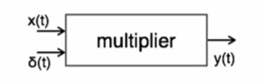
- Sampling is a process performed by a sampler
- Analog signal is samples every secs, called sampling interval.
- Sampling rate/ frequency =
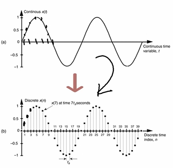
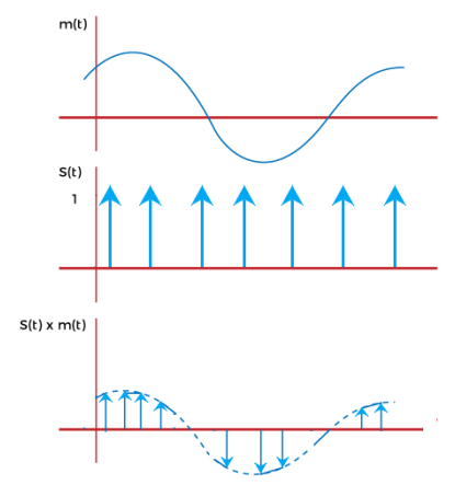
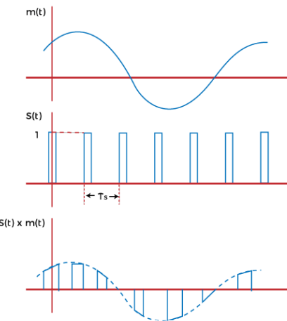
When the continuous signal is sampled at regular intervals multiplied by a periodic pulse train / impulse train , the produced signal is the sampled signal.
Sampling Theorem: A continuous time signal can be represented in its samples and can be recovered back when sampling frequency is greater than or equal to the twice highest frequency component of message signal.
[]
Condition:
Sampling rate is defined as the number of samples taken per second from a continuous signal for a finite set of values.
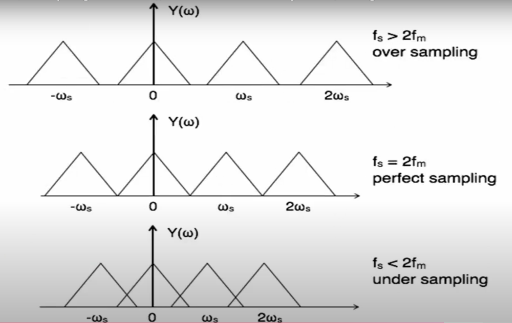
Nyquist rate: The theoretical minimum sampling rate /inline eq at which a signal can be sampled and still can be reconstruct samples without any distortion.
Nyquist Interval: Nyquist interval is the reciprocal of the Nyquist rate.
Methods of Sampling
- Ideal Sampling
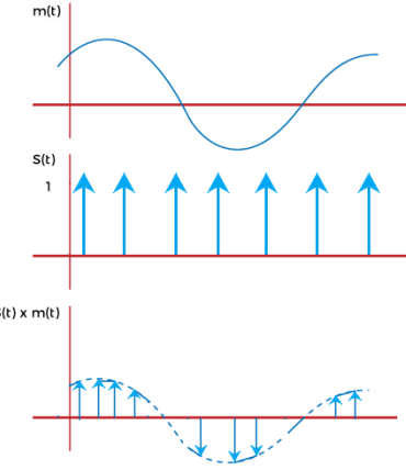
- Known as instantaneous sampling/impulse sampling
- multiplied by a impulse train signal
- Sampling rate in infinite
- Bandwidth is large
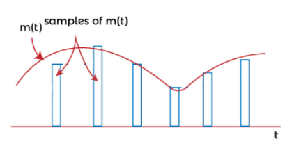
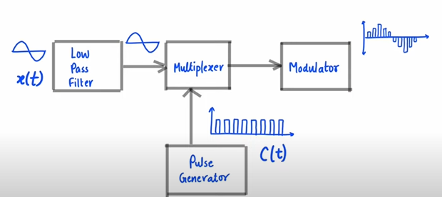
- Natural Sampling
- considered as efficient multiplexing method in Pulse Amplitude Modulation
- multiplied by the uniformly spaced rectangular pulses
- pulses do not have flat tops, they are curved
- their tops follow the waveform of input or message signal
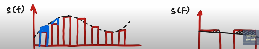
- Flat-top Sampling
- easier than natural sampling
- amplitude of sampled pulses are constant
- pulses have flat top
- Aperture effect: The loss of high frequency content because of constant amplitude. Example:
Advantages/Why
The advantages of the sampling process are due to conversation of the transmission of digital form, which have various advantages.
Applications: PAM, PCM, TDM
- Low cost
- High Accuracy
- Easy to implement
- Less time consuming
- Low signal loss
- High Scope
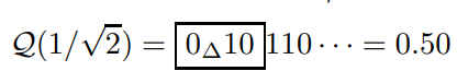
Quantization
Quantization is the process in which continuous amplitude (analog) signals is converted into discrete amplitude (digital) signals.
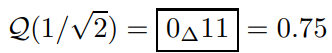
Given a real number m we denote the quantized value of as,
, where is the quantization error.
There are two main types of quantization
- Truncation
Just discard the least significant bits
- Rounding
just choose the closet value
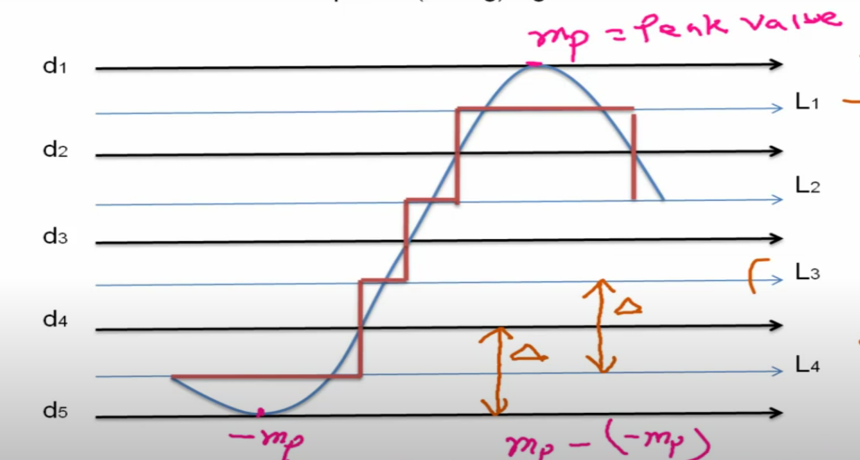
Peak to peak value =
- Dividing by decision boundaries (Here 5)
- Quantization level () : Decision Boundaries - 1
- Step size,
- Number of bits to represent each sample (Level),
Quantization Error: The difference between an input and output of a quantizer is known as a quantization error.
Quantization Error,
Range of quantization error :
Signal-to-noise Ration
,
Unit : Watt or ,
Signal Power,
Quantization noise power/ Average Quantization power / Mean square value of quantization error ,
Noise power, [Derivation below]
[ ]
Bit Rate: The total bits transmitted in one unit time. It means the total bits that travel per second.
, Unit : , bits per second
Shannon Capacity or Channel Capacity: Shannon’s Channel Capacity theorem states that the maximum rate at which information can be transmitted over a communication channel of a specified bandwidth in the presence of noise.
It tells us the theoretical highest limit in which any channel can transmit signals with the presence of noise. [Ref]
Baud Rate: The total number of signal units transmitted in one second.
| Parameters | Baud Rate | Bit Rate |
|---|---|---|
| Basics | The Baud rate refers to the total number of signal units transmitted in one second. | The Bit rate refers to the total Bits transmitted in one unit time. |
| Meaning | Baud rate indicates the total number of times the overall state of a given signal changes/ alters. | Bit rate indicates the total bits that travel per second. |
| Determination of Bandwidth | The Baud rate can easily determine the overall bandwidth that one might require to send a signal. | The bit rate cannot determine the overall signal bandwidth. |
| Generally Used | It mainly concerns the transmission of data over a given channel. | It mainly focuses on the efficiency of a computer. |
| Equation | Baud Rate = Rb/n | Bit Rate = fs * n |
[Ref]
Pulse Code Modulation (PCM)
Information is transmitted in the form of “code words”. PCM output is in coded digital form.
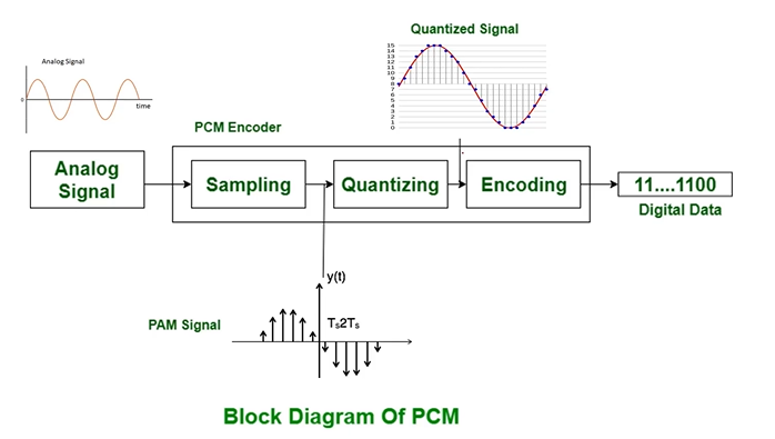
- LPF
- Bandlimits
- Eliminates possibility of aliasing
- Encoder
- Analog to digital converted
- Each quantized level convert into N bit digital word
- Sample & Head Circuit
- Convert to flat top PAM
- Parallel to Serial Converter
- Quantizer
- Quantized PAM
Decoder
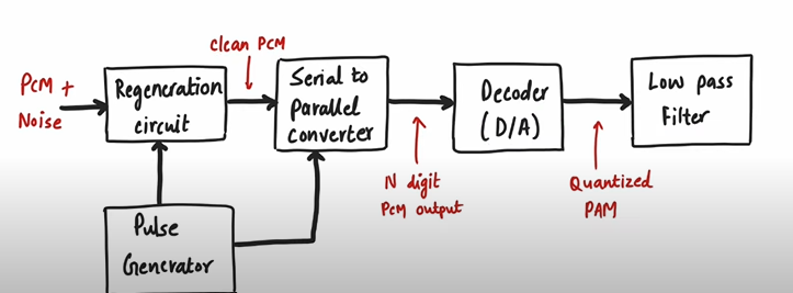
Advantages
- Very high noise immunity
- Due to digital nature of the signal, repeaters can be placed between transmitter and receiver. It reduce the effect of noise and regenerate the received PCM signal.
- It is possible to store PCM.
- It is possible to use various coding techniques so that the desired person can decode the received signal.
- Integration with other form of digital data is possible
Disadvantages
- The encoding, decoding and quantizing circuitry of PCM is complex.
- Requires a large bandwidth
Applications:
- Telephony
- Space Communication (because of high noise immunity)
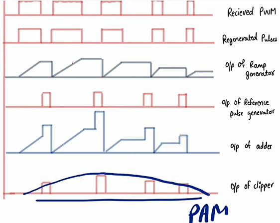
Pulse Amplitude Modulation
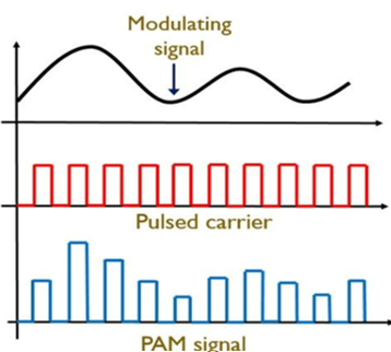
- amplitude of the pulse carrier signal is changed according to the amplitude of the message signal.
- Sampling Method: Flat Top PAM, Natural PAM
Applications: Ethernet, Photo biology, Driver for LED lighting, Micro controller
Demodulation
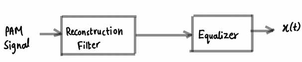
Reconstruction Filter:
- Cut off frequency
Equalizer:
- Reduce aperture effect and attenuation
Advantages
- Simple modulation and demodulation
- No complex circuitry for transmission and reception
- PAM can generate other pulse modulation
- Can carry message or information at the same time
Disadvantages
- Bandwidth will be large. Due to Nyquist criteria also high bandwidth is required.
- Amplitude varies according to modulating signal → interference → more noise
- Pulse amplitude signal varies → more power required
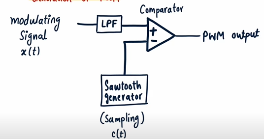
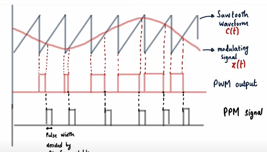
Pulse Width Modulation (PWM)
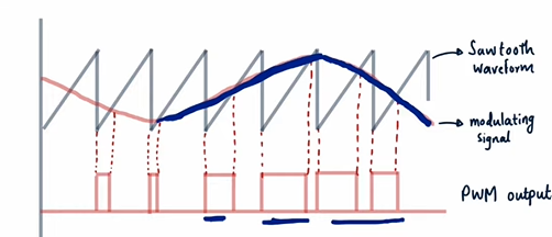
- Amplitude of → Width of PWM Signal
- Amplitude of → Width of PWM Signal
- Leading edges of PWM waveform coincide with the falling edges of ramp signal
Comparator
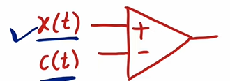
- Output High,
- Output Low,
Generation of PWM
- non-inverting
- inverting
Demodulation
Advantages
- Amplitude constant → Noise interference less
- Signal and noise can be separated very easily at demodulation
- Synchronization between transmitter and receiver is not requires
Disadvantages
- Power will be variable → width of the pulse varies
- Bandwidth is large compared to PAM
Applications: Telecommunication, robotics, audio effects and amplifications, control the amount of power, control the speed of the robot
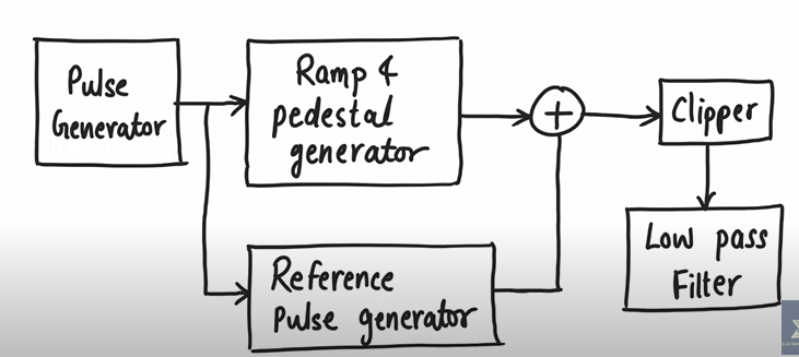
Pulse Position Modulation (PPM)
Position of pulse varies according to modulating signal.
PPM can be derived from PWM.
Generation
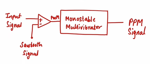
Monostable:
- One stable state (Low)
- Give Trigger pulse → output = High (for some time)
- “Some time” depends on Register and Capacitor (RC) component
- Width and Amplitude Constant
- Position varies
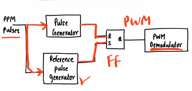
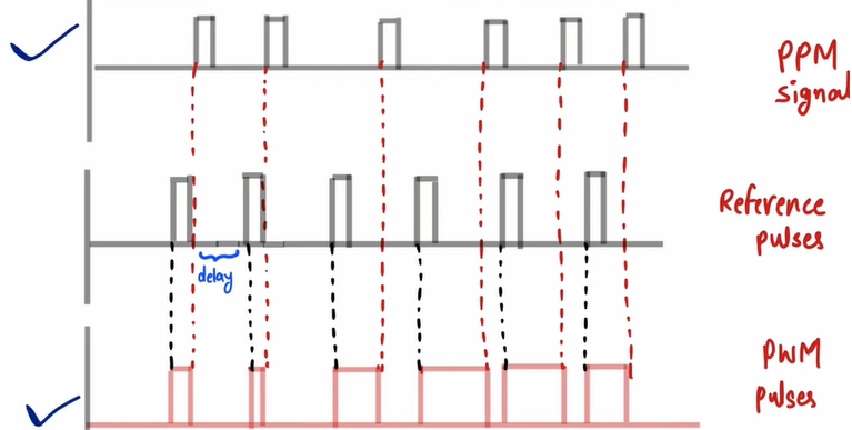
Demodulation
Advantages
- Low noise interference compared to PAM
- Noise removal and separation is very easy
- Power usage is very low
Disadvantages
- Synchronization between transmitter and receiver is required.
- Large bandwidth
Applications: Non coherent detection, RF communication, contactless smart card, RFID