Artificial Intelligence
| Created by | Borhan |
|---|---|
| Last edited time | |
| Tag |
Resources
- Atkia Apu’s Note
- Mahir Labib Dihan Sir’s Note
Introduction to AI, Turing test, Agents
Artificial Intelligence (AI) is a branch of computer science and engineering that deals with intelligent behavior, learning, and adaptation in machines.
Views of AI fall in four categories:
- Thinking humanly
- Thinking rationally
- Acting humanly
- Acting rationally
Turing Test: A computer passes the test if a human interrogator, after posing some written questions, cannot tell whether the written responses come from a person or a from a computer.
Capabilities of passing Turing test
- Natural language processing to enable it to communicate successfully in English.
- Knowledge representation to store what it knows or hears.
- Automated reasoning to use the stored information to answer questions and draw new conclusions.
- Machine learning to adopt to new circumstances and to detect and extrapolate patterns.
Agents: An agent is anything that perceives its environment through sensors and acts upon it through actuators.
Structure
- Sensors: Devices that collect environmental data
- Percepts: Data received from sensors
- Actuators: Mechanisms that allow the agent to act on the environment
- Actions: Tasks performed by actuators
Types of Agents
| Agent Type | Description | Key Features | Limitations | Example |
|---|---|---|---|---|
| Simple Reflex Agent | Acts based on current percepts, using condition-action rules ("If X, then Y"). | No memory of past percepts; simple to implement. | Limited intelligence; may enter deadlocks or loops. | Thermostat turning on/off based on temperature. |
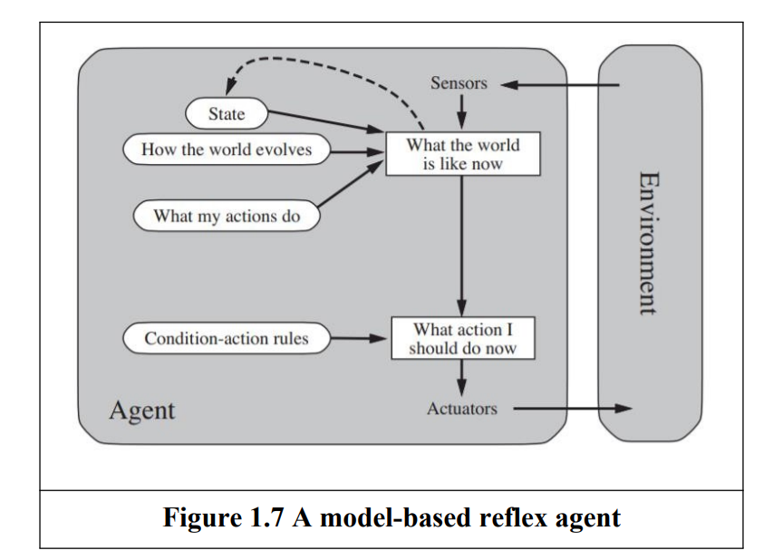
| Model-Based Reflex Agent | Maintains an internal state to track unobserved environment aspects. | Uses knowledge of world evolution and action effects. | Requires modeling of environment dynamics. | Robot navigating a partially visible room. |
| Goal-Based Agent | Acts to achieve specific goals by evaluating action sequences. | Flexible; explicit knowledge representation. | Requires search/planning for goal achievement. | Navigation system planning a route. |
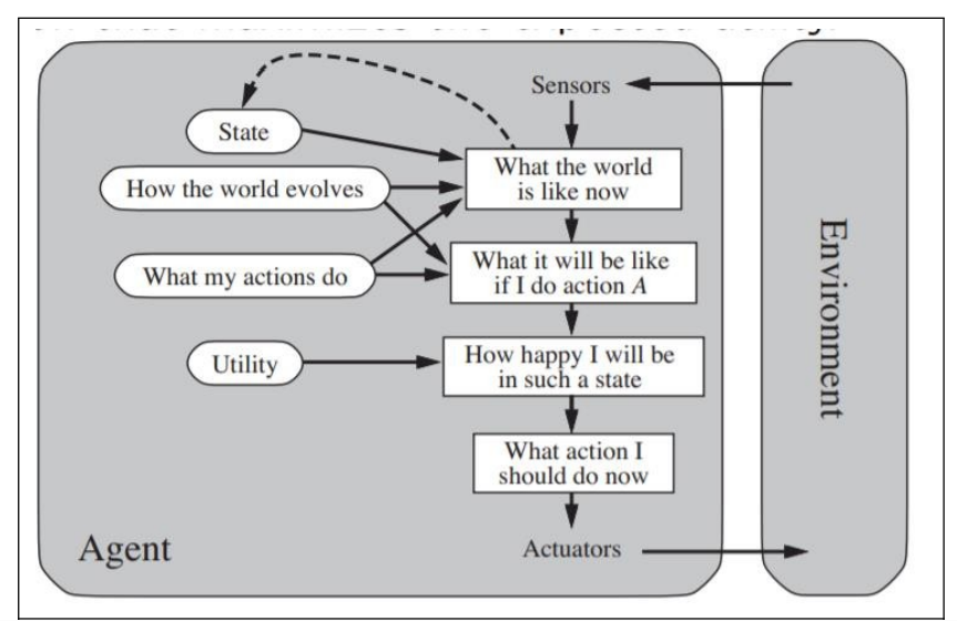
| Utility-Based Agent | Chooses actions based on a utility function measuring success. The Utility-based agent is useful when there are multiple possible alternatives, and an agent has to choose in order to perform the best action. | Balances conflicting goals and success likelihood. | Complex to compute utility for all states. | Robot prioritizing speed vs. safety. |
| Learning Agent | Learns from experience to improve performance. | Components: Learning Element, Performance Element, Critic, Problem Generator. | Needs initial knowledge; learning takes time. | Self-driving car adapting to traffic patterns. |
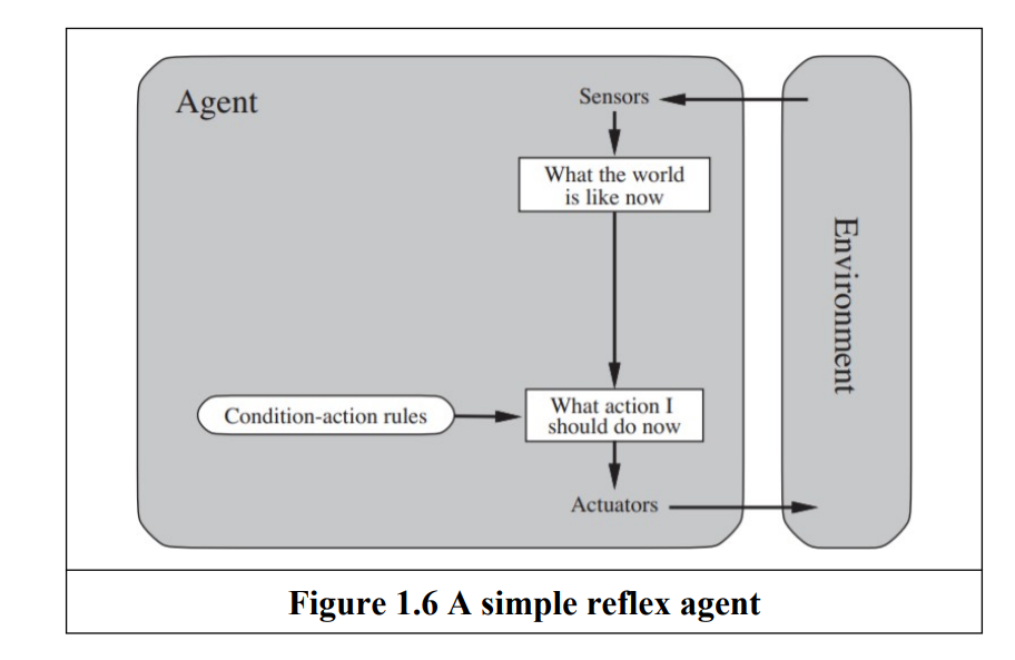
- Reflexive Agent: An agent whose action depends only on the current percepts.
- Model based : An agent whose action is derived from an internal model of the current world state
- Partial observability
- Updating the internal state information as times goes by requires two kinds of knowledge to be encoded
- We need some information information about how the world evolves independently of the agent
- We need some information about how the agent’s own actions affect the world
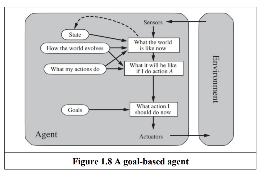
- Goal Based agent : An agent that select actions that it believes will achieve explicitly represented goals.
- Expansion of Model based agent
- Desirable situation
- Searching and planning
- Utility Based Agent: An agent that selects actions that it believes will maximize the expected utility outcome state
- Utility function
- Deals with happy and unhappy state
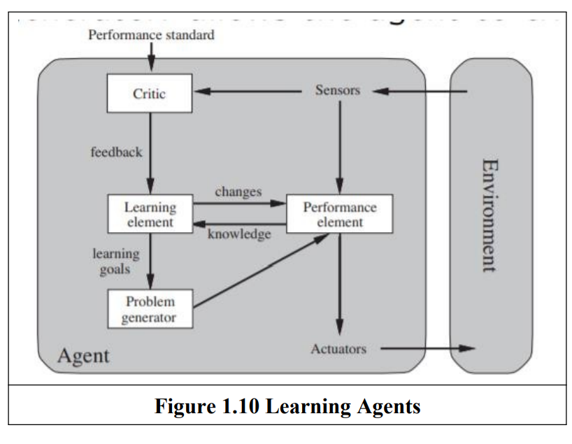
- Learning Agent: An agent whose behavior improves over time based on its experience
- Learning Element: Responsible for making improvements.
- Performance Element : is what we have previously considered to be the entire agent: it takes in percepts and decides on actions
- Critic: The learning element uses feedback from the critic on how the agent is doing and determines how the performance element should be modified to do better in the future.
- Problem Generator: suggesting actions that will lead to new and informative experiences.
- Rational Agent: A rational agent selects actions that maximize its performance measure, based on percepts and build-in knowledge.
- act to gather information or explore for better outcomes
- autonomous if their behavior is based on their own experience
- Rationality does not imply omniscience
- Autonomous Agents: Agents whose behavior is determined by their own experience rather than pre-programmed decisions.
- Sufficient initial knowledge to operate
- Ability to learn and adapt to new situations
- Omniscience: An omniscient agent knows the exact outcomes of its actions and its certain no other outcomes are possible.
- It is impossible in real-world
Different informed and uninformed search techniques
State space search: It is the possible of all states including start and goal state where a particular problem solution is going to be searched.
Data structure: Graph
Represented By
- A set of states
- An initial state
- A set of operators or actions
- A partial function/transition function
- A set of goal states
- An optional path cost function
Generalized state space search algorithm
Initialize:
	L : Linked List = {}
	Sc : Node = Null
	GOAL_FOUND : Boolean = FALSE
	GOAL_EXISTS : Boolean = TRUE

Add node si (intial) to L
WHILE GOAL_FOUND IS FALSE
AND GOAL_EXISTS IS TRUE
DO
	SET Sc : An unexpanded node from L
	IF Sc IS NOT NULL THEN
		FOREACH successor node Ss of Sc DO
			IF Ss EQUALS Sg THEN
				SET GOAL_FOUND = TRUE
			ELSE
				IF L not contains Ss THEN
					Add Ss to L
				END IF
			END IF
			MARK Sc as expanded
		END FOREACH
	ELSE
		SET GOAL_EXISTS = FALSE
	END IF
END WHILE
Search Tree:
- State space represented by Search Tree.
- A fundamental data structure that used to systematically represent and explore all possible search states of a problem to find a solution.
- Provides a framework for solving problems by simulating the decision making process through a sequence of actions.
- In search tree
- A root node represents the initial state
- Children of a node → successor
- Fringe of a tree → States not yet expanded
Properties we use to evaluate an algorithm
- Completeness : Guaranteed to find a solution if one exists
- Optimal : If it always find the best solution
- Time complexity: The amount of time an algorithm takes
- Space Complexity : The amount of memory an algorithm requires
Informed vs Uninformed
| Aspects | Uninformed | Informed |
|---|---|---|
| Definition | Search algorithm that explore the problem space without any domain-specific knowledge or heuristics, relying on problem structure and predefined rules. Also known as blind search algorithm. | Search algorithms that use domain-specific heuristic or estimates of the cost to reach the goal. |
| Knowledge Used | Only problem structure | Heuristics estimate cost to goal. |
| Time | Consuming | Quick Solution |
| Cost | Costly | Less |
| Time and Space Complexity | More | Less |
| Example | BFS, DFS | A*, Best first search |
Uninformed Algorithm
- Breadth-First-Search Algorithm
- Explores all nodes at the current depth before moving to the next level
- Uses a queue FIFO
- Shortest path but more memory
- Depth-First-Search
- Explores as far as possible along each path before backtracking
- Uses a Stack LIFO
- Infinite loop, memory-efficient
- How it detects cycle
- When DFS is applied over a graph if DFS finds an edge that points to an already visited vertex
- DFS is not optimal
- Doesn’t consider path cost
- Many states keep reoccurring → No guarantee to find a solution
- May go to infinite loop
- Doesn’t find the shortest path always
- Depth Limited Search
- A variation of DFS that limits the depth of exploration to prevent infinite loops in large or infinite space spaces
- Useful when the goal depth is known but cannot find solution beyond the depth limit.
- Limitation
- Not optimal
- Incompleteness
- Effectiveness depend on the depth limit
- Iterative Deepening Depth First Search
- combines BFS and DFS altogether
- Adv
- Ensure completeness and optimally → BFS
- Memory Efficient → DFS
- Dis
- repeats all the work of the previous phase
- Uniform Cost Search
- Extends BFS by considering path costs always expanding the last cost node first.
- Find the least cost, Slower than BFS
- Bidirectional Search
- Runs two simultaneous searching one from initial state (forward search) and another from goal (backward search)
- It replaces one search graph with two small search subgraphs
- The search stops when there two graphs intersect each other
- When it doesn’t work
- Implementation of tree is difficult
- The goal state is unknown/unclear in advance
- Finding an efficient way to check if a match exists is tricky which can increase the time.
| Algorithm | TC | SC | Optimal | Complete |
|---|---|---|---|---|
| BFS | b^d | b^d | Yes | Yes |
| DFS | b^d | bd | No | No |
| DLS | b^l | bl | No | if l ≥ d |
| IDDFS | b^d | bd | Yes | Yes |
| Uniform | b^d | b^d | Yes | Yes |
| Bidirectional | b^(d/2) | b^(d/2) | Yes | Yes |
Informed Search, Heuristics*, How heuristics help? A* search, Proof of optimality of A*
https://iipseries.org/assets/docupload/rsl2024AF233C7BF02A178.pdf
- Best-First Search
- Greedy search, It picks such path that appears best at the moment.
- A blend of both DFS and BFS
- Choose the most promising node at each step
- It is applied by priority queue
- Advantage :
- It switch between BFS and DFS by gaining the advantage of both algorithm
- More effective and capable than BFS, DFS
- Disadvantage
- Worst scenario : operate as an unguided DFS
- Get stuck in a loop
- Not optimal
- Not complete
- TC/SC :
- A* Algorithm
- Heuristic : A heuristic is a technique designed to solve a problem faster than classic method or to find an approximate solution when the classic methods fail to find any exact solution.
- How it helps in finding solution
- It useful in reducing the time and resources required to find the solutions by focusing the search on the most promising path.
- It prioritizes which node to explore based on their estimated cost to the goal.
- It helps in state space search by guiding the exploration, reducing the search space and improving efficiency.
- It allows algorithm to focus on exploring path that are more likely to be solution.
- Admissible Heuristic: A heuristic is admissible if for every node , , where is the true cost to reach the goal statement from . An admissible heuristic never overestimates the cost to reach the goal, thus it is optimistic.
- for all node and both are admissible then dominates . is better for search.
- How it helps in finding solution
- Evaluation Function,
- Optimal, Complete
- TC : Exponential.
- is always optimal
Suppose some suboptimal goal has been generated and is in the fringe. Let n be an unexpanded node in the fringe such that n is on a shortest path to an optimal goal .
A* will never select for expansion.
A heuristic is consistent if for every node n, every successor n’ of n generated by any action a,
If h is consistent,
is non-decreasing along any path. So, A* using graph search is optimal.
- Prove that the uniform-cost search is a special case of A* search.
A* search uses the evaluation function:
where:
-
-
Uniform-Cost Search (UCS) does not use a heuristic, so:
Therefore, for UCS, the evaluation function becomes:
This means UCS always expands the node with the lowest path cost g(n), exactly like A* with a zero heuristic.
Hence, Uniform-Cost Search is a special case of A Search where the heuristic function h(n)is zero for all nodes.
g. Prove that, if heuristic function h never overestimates by more than cost c, A* using h returns a solution whose cost exceeds that of the optimal solution by no more that c.
Now, suppose h(n) <= h*(n)+c as given and let G2 be a goal that is sub-optimal by more than c, i.e. f(G2)=g(G2) > C* +c. Now consider any node n on a path to an optimal goal. We have
f(n)=g(n)+h(n) <= g(n)+h*(n)+c <= C*+c <= f(G2)
so G2 will never be expanded before an optimal node is expanded
because f(n)<f(G2)
- Heuristic : A heuristic is a technique designed to solve a problem faster than classic method or to find an approximate solution when the classic methods fail to find any exact solution.
Local Search Algorithm: Local search algorithms are essential tools in artificial intelligence and optimization, employed to find high-quality solutions in large and complex problem spaces.
- Hill-Climbing Search:
- It is a straightforward local search algorithm that iteratively moves towards better solution.
- Process : Start → Evaluate → Move → Repeat
- Pros: Easy to implement, works well in small search space
- Cons
- Local Maxima: Hill-climbing can get stuck at a local maximum.
- Plateaus: On a flat region where neighboring states have the same heuristic value, hill-climbing may wander aimlessly, slowing progress or failing to find the goal.
- Ridges: In state spaces with ridges (narrow paths of improvement), hill-climbing may oscillate between states without advancing toward the goal.
- No Backtracking: Hill-climbing only considers the current state and its neighbors, without backtracking to explore alternative paths, missing better solutions elsewhere.
- Solution
- Introduce Gradient descent search which is a variation of all hill climbing that moves downhill
- Introduce a small random jump to escape the plateau.
- Use stochastic hill climbing where steps are probabilistic can help navigation ridges.
- Simulated Annealing
- Local Beam Search
- Genetic Algorithm
- Tabu Search
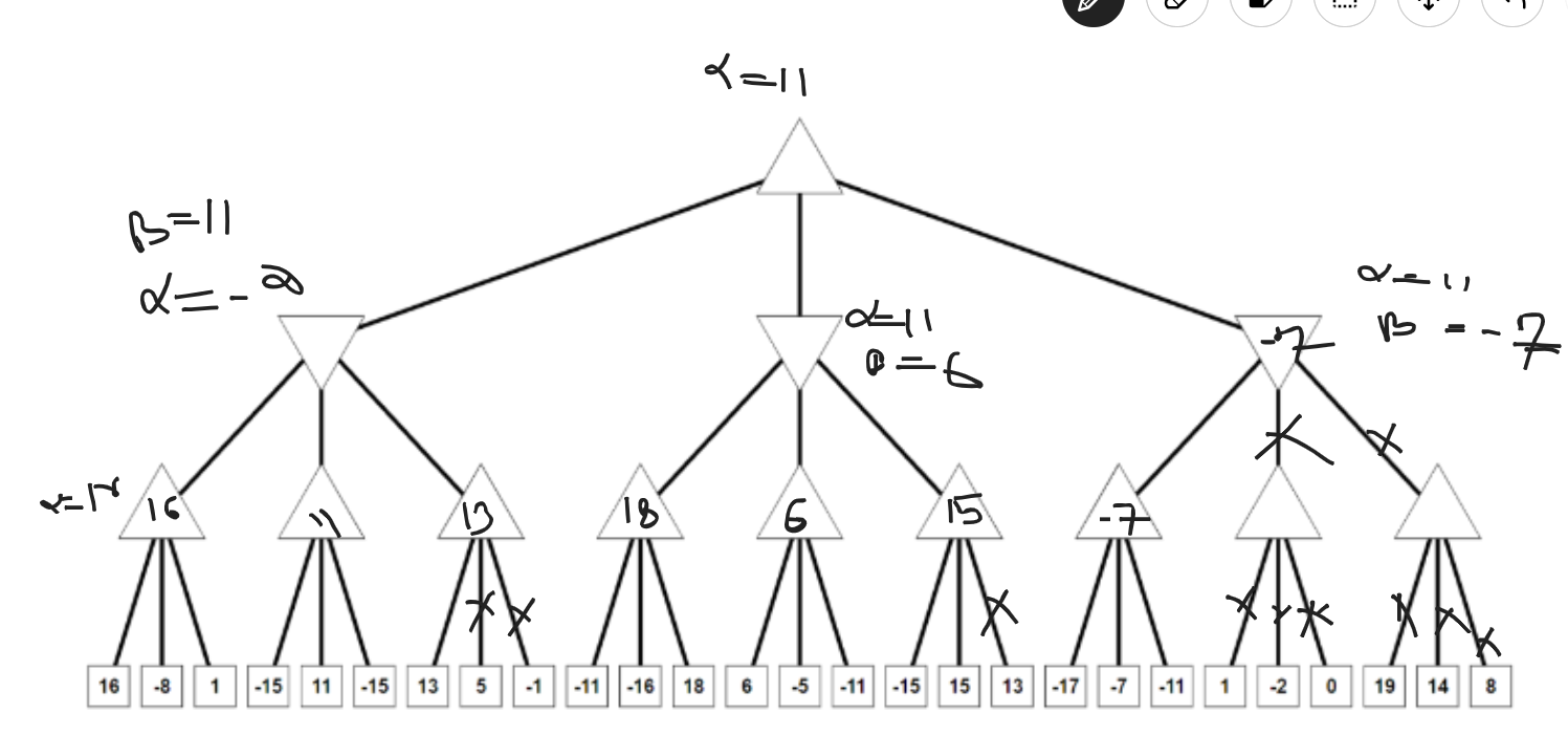
2 player zero sum games, mini-max algorithm, alpha-beta pruning
https://www.arsdcollege.ac.in/wp-content/uploads/2020/03/Artificial_Intelligence-week3.pdf
The 2-person 0-sum game is a basic model in game theory. There are two players, each with associated set of strategies. While one player aims to maximize his payoff, the other player player attempts to take an action to minimize this payoff. The gain of a player is the loss of another.
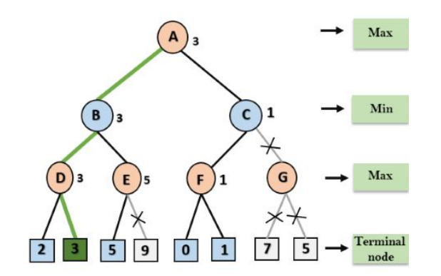
Mini-Max Algorithm
Mini-max algorithm is a recursive or backtracking algorithm which is used in decision making and game theory.
- Both opponent plays optimally
- Both the players fight it as opponent player gets the minimum benefit while they get the maximum benefit.
- MAX will select maximized value
- MIN will select the minimized value
- A DFS algorithm
- Proceed all the way down to the terminal node then backtrack the tree as recursion.
The game is modeled as a game tree
- Node → Game State
- Edges → Legal Moves
- Root → Current Position
- Leaves → Game Outcomes with utility value (+1 → max, -1 → min)
Process
- Start at the root (MAX turn)
- Recursively, explore all possible moves down to terminal nodes or fixed depth
- At leaf node assign values using a utility function or heuristic evaluation function for non-terminals states
- Backpropagate values
- At max nodes → Select he child with highest value
- At min Nodes → Select the child with lowest value
- At the root, choose the move that yields the highest value ensuring the best outcome against min optimal play.
Analytics:
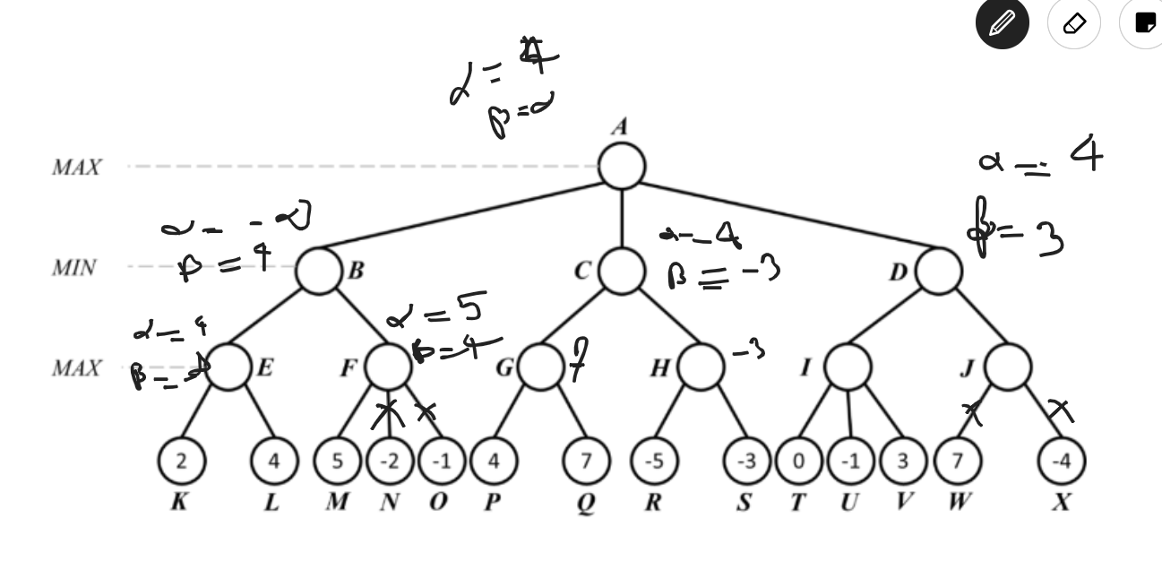
Alpha-beta Pruning
- Modified version of minmax algorithm
- It uses an optimization technique for the minimax algorithm.
- The alpha-beta pruning to a standard minimax algorithm returns the same move as the standard does, but it removes all the nodes which are not really affecting the final decision but making algorithm slow.
- Alpha : The best/highest-value choice we have found so far at any point along the path of maximizer. Initial value of a alpha is
- Beta: The best/lowest-value choice we have found so far at any point along the path of minimizer. The initial value is
- Condition for alpha-beta pruning
-
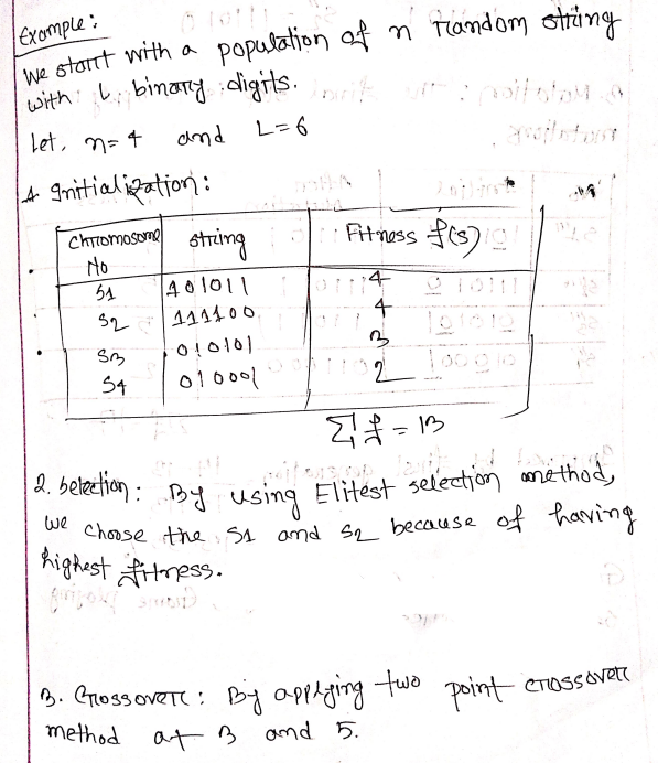
Genetic algorithm, steps of genetic algorithm. (using MAXONE problem, see slides), Different Crossover and Selection techniques, GA for solving optimization problems
https://egyankosh.ac.in/bitstream/123456789/12697/1/Unit-11.pdf
http://www.cs.cmu.edu/~02317/slides/lec_8.pdf
Genetic Algorithm: A genetic Algorithm is a search heuristic inspired by Charles Darwin’s “Theory of Natural Evolution”. IT is used to solve optimization problem by mimicking the process of natural selection where the fittest individual are selected for reproduction to produce offspring for the next generation.
Application of GA: Optimization, Automatic Programming, Machine and robot learning, Economic models, Ecological models, Population genetic models and Models of social systems.
Steps
- Initialization: Start with randomly generated population
- Evaluation: Evaluate each individual using a fittest function
- Selection: Select the individuals for reproduction using different techniques
- Types of selection techniques
- Roulette Wheel Selection: Conceptually, this can be represented as a game of roulette - each individual gets a slice of the wheel, but more fit ones get larger slices than less fit ones.
- Rank based selection: where the probability of an individual being selected for reproduction or survival is determined by its rank within the population, not its raw fitness score.
- Elitist Selection: Chose only the most fit members of each generation.
- Cutoff Selection: Select only those that are above a certain cutoff for the target function.
- Scaling Selection :
- Roulette Wheel Selection: Conceptually, this can be represented as a game of roulette - each individual gets a slice of the wheel, but more fit ones get larger slices than less fit ones.
- Types of selection techniques
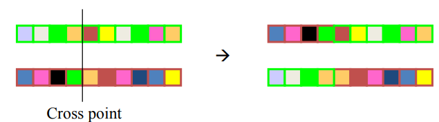
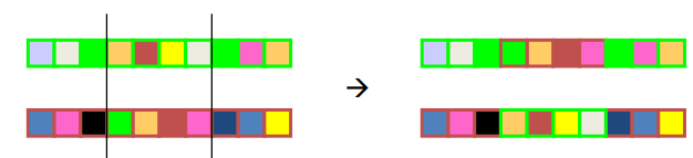
- Crossover: Combine pair to produce offspring
- Types
- Single Point: Randomly select a single point for a crossover
- Two point crossover: Avoids cases where genes at the beginning and end of a chromosome are always split
- Uniform
- A random subset is chosen
- The subset is taken from parent 1 and the other bits from parent 2
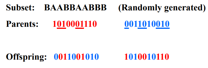
- Types
- Mutation : Random changes to some individual to maintain diversity
- Mutation prevents the algorithm to be trapped in a local minimum
- Termination: Repeat the process until the criterion met
The basic algorithm
- [Start] Genetic random population of n chromosomes
- [Fitness] Evaluate the fitness of each chromosome x in the population
- [New Population] Create a new population by repeating following steps until the New Population is complete
- [Selection] Select two parent chromosomes from a population according to their fitness value
- [Crossover] With a crossover probability, cross over the parents to form a new offspring.
- [Mutation] With a mutation probability, mutate new offspring at each locus.
- [Accepting] Place new offspring in the new population
- [Replace] Use new generated population for a further sum of the algorithm
- [Test] If the condition is satisfied, stop and return the best solution in current population.
- [Loop] Go to Step2 for fittest evaluation.
MaxOne problem: The Maxone problem is to find a binary string of length ‘l’ that contains the maximum number of one. The optimal solution is a string of all 1s.
Bayes' rule, Belief update*, Naive Bayes Classifier, Formulation, Dealing with sparse data, Usage in document classification*, Gaussian Naive Bayes
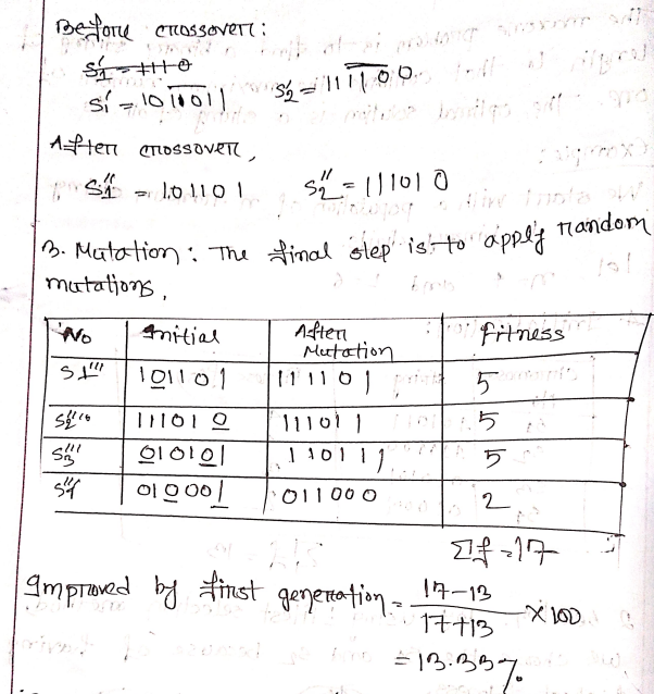
Baye’s Theorem: Baye’s theorem is a fundamental principle in probability theory that allows for the computation of the conditional probability of a hypothesis H gives observed evidence E.
Derivation:
⇒
⇒
⇒
Bayesian Network: It is a decision making tool . A BN is a powerful probabilistic graphical model used for decision making under uncertainty,
Principle:
- Structure: It consists of DAG and CPT (Conditional Probability Tree)
- Node : Random Variable
- Edge : Conditional Dependency
- No Edge : Conditional Independence.
Each node associated with a CPT that quantifies the probability of the node given its parent node.
The network encodes the joint probability distribution of all variables as
- Probabilistic Inference : BN update the probabilities of known variable using Baye’s theorem, facilitating reasoning under uncertainity. For example, the network can be used to update knowledge of the state of a subset of variables when other variables (the evidence variables) are observed. This process of computing the posterior distribution of variables given evidence is called probabilistic inference.
- Belief Update: A Bayesian update or belief update is a change in probabilistic beliefs after gaining new knowledge. For example, after observing a patient's test result, we might revise our probability that a patient has a certain disease. If this belief revision obeys Bayes's Rule, then it is called Bayesian. When the evidence is observed, the prior probabilities are update to posterior probabilities.
Application: Medical diagnosis, decision support, prediction and forecasting, anomaly detection.
Naive Bayes Classifier: Naive Bayes is a classification algorithm that uses probability to predict which category a data point belongs to, assuming that all features are unrelated.
Formulation
Bayes theorem,
C : Class, X : Feature
Naive assumption: All features are conditionally independent given the class.
Hence, final classification becomes,
Dealing with Sparse Data (Zero Probabilistic)
In real datasets, some feature-class combinations may not appear in training data, resulting in zero probability, which can nullify the whole product.
To handle this, we use Laplace Smoothing (Additive Smoothing):
Usage in document classification
Spam filtering, sentiment analysis, topic classification
Definitions
- Mass function: The mass function, denoted , assign a value range to every subset frame of discernment.
- Belief (Bel): The belief function, , for a subset A is the sum of the mass probabilities of all proper subset of A.
- Plausibility (Pls): The plausibility function, , represents the maximum possible belief in A.
- Belief Interval : The belief interval for a subset A is the range , which express the range of belief in A.
Gaussian Naive Bayes Algorithm
Gaussian Naive Bayes is a type of Naive Bayes method working on continuous attributes and the data features that follows Gaussian distribution throughout the dataset.
- Calculate Mean and Variance
-
-
Decision Tree, Information Gain & Gini Index.
A decision tree is a machine learning model that uses a tree like structure to make decision based on a sequence of questions and conditions.
Entropy is a measure of impurity or disorder in a dataset
Information Gain measures the reduction in entropy after a dataset is split on an attribute:
Gini Index :
Machine Learning, Steps of ML, Hyperparameter tuning, why needed?
https://www.cs.cmu.edu/~hn1/documents/machine-learning/notes.pdf
Machine learning is programming computers to optimize a performance criterion using example data or past experience.
| Aspect | Traditional Programming | Machine Learning |
|---|---|---|
| Programming | Rules and logic are manually coded by the programmer. | Model learns patterns automatically from data. |
| Input | Data and explicit rules. | Data (often labeled for supervised learning). |
| Output | Deterministic output based on coded rules. | Predictions or decisions based on learned patterns. |
| Flexibility | Limited to predefined rules; changes require recoding. | Adapts to new data; retraining updates the model. |
| Use Cases | Well-defined, rule-based tasks (e.g., payroll, sorting). | Complex, pattern-based tasks (e.g., image recognition, predictions). |
| Examples (Lecture 1) | Calculating payroll | Speech recognition, personalized |
Steps of ML
- Project Setup : This is the first step to plan and set up the environment for machine learning project.
- Understand Business Goal
- Having conversation with stakeholders
- Choose the solution to the problem
- Which category of the models derive the highest impact
- Understand Business Goal
- Data Preparation:
- Collection of data
- Clear about the goal with clear objective → Identify which data are vital for the model tuning
- Collecting related data from various sources according to project requirement
- Cleaning of Data
- Identify and handle missing values, inconsistencies, removing duplicates
- Data transformation
- Convert cleaned data into a format suitable for machine learning
- modifying or converting data, feature scaling, feature encoding
- Data Reduction
- Simplifying data without losing the essence
- Data Splitting
- Split data into different sets to ensure more reliable and actionable
- Splitting of data
- Training set:
- actual dataset from which a model trains
- model sees and learns from this data
- 60% of total data
- Validation set
- Used to training hyperparameters
- Model sees this data for evaluation but doesn’t learn from this
- 15% of total data
- Testing set
- Evaluate the model after training to complete
- Provides unbiased evaluation of the models
- 20-25% of data
- Training set:
- Importance of data preparation
- Provide reliable prediction outcomes
- Identify data issues or error
- Increase decision making capability
- Reduce cost
- Increase model performance
- Collection of data
- Deployment:
- Deploy the model:
- integrating it into a production environment where it can process real world data
- MLOPS
- Monitor Model performance
- Regularly test the performance of model as data
- Improve Model
- Continuously iterate and improve model
- Replace model with an updated version
- Deploy the model:
| Feature | Random Split | Stratified Split | K-Fold Cross-Validation | Time-Based Split |
|---|---|---|---|---|
| How it works | Randomly divides data | Keeps class proportions same | Splits data into k parts, trains k times. in each iteration, k-1 folds are used for training, and the remaining 1 fold is used for validation | Splits data by time order. Earlier data points form the training set, and later data points form the test or validation set |
| When to use | Data has no order, balanced classes | Classification with imbalanced classes | When data is small, want reliable results | For time-series or sequential data |
| Pros | Simple and fast | Keeps classes balanced | Uses all data for training and testing | Keeps time order, avoids future data leaking |
| Cons | May not keep class balance | Only for classification problems | Takes more time to run | Not for random data, only ordered data |
| Example | Splitting customer data randomly | Heart disease data with rare cases | Small dataset with 5 folds | Stock prices split by date |
Hyperparameter
Hyperparameter tuning is a fundamental process in machine learning that involves selecting the best set of hyperparameters to maximize a model's performance and generalization ability. Hyperparameters are predefined configuration settings, such as learning rate, batch size, or the number of layers, which are not learned from the data but significantly influence the training process and final model quality.
Some techniques
- Grid Search : exhaustively tests all combinations of specified hyperparameter values
- Random Search: which samples parameter combinations randomly to reduce computation cost
Importance of it
- Improve model performance: capturing patterns without overfitting or underfitting
- Balance bias and variance trade off: controls complexity that affects the bias-variance trade off.
- Enhancing learning efficiency
- Optimizes resource usage:
Supervised, Unsupervised and Reinforcement learning
| Aspect | Supervised Learning | Unsupervised Learning | Reinforcement Learning |
|---|---|---|---|
| Definition | A model is trained on a labeled dataset with input-output pairs to predict outputs for new data | A model identifies patterns or structures in unlabeled data without predefined outputs | An agent learns by interacting with an environment, making decisions to maximize cumulative rewards . |
| Data Type | Labeled (input-output pairs) | Unlabeled (no predefined outputs) | No predefined input-output; uses rewards |
| Goal | Predict accurate outputs for new inputs | Find patterns or structures in data | Maximize cumulative reward |
| Feedback | Direct (correct labels) | None (inferred from data structure) | Delayed (reward signals from environment) |
| Examples | House price prediction, disease classification | Customer segmentation, data compression | Robot navigation, game playing |
| Algorithms | Linear regression, SVM, logistic regression | K-means, PCA | Q-learning, policy gradients |
| Human Involvement | Yes | No | Low |
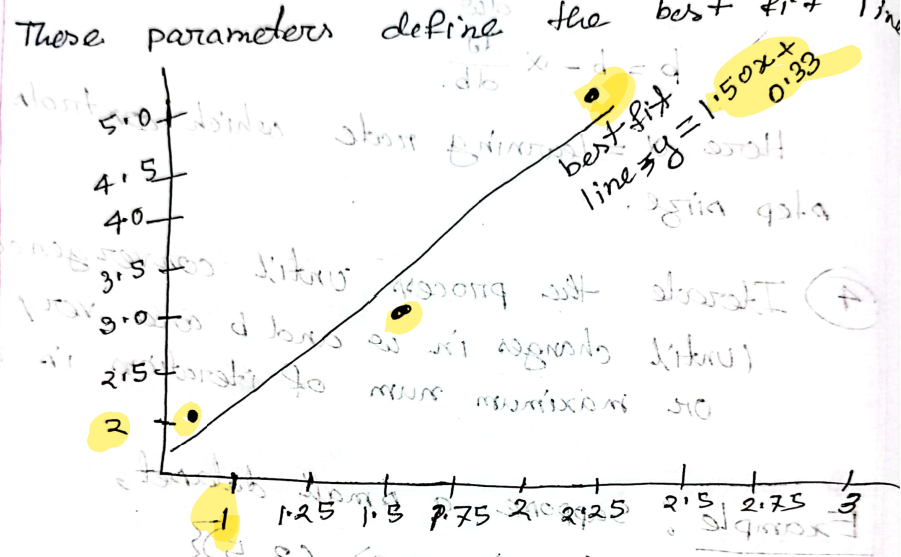
Gradient Descent Algorithm using a linear regression example
Gradient Descent is an optimization algorithm used to find the optimal parameters of a machine learning model by iteratively adjusting parameters to minimize.
In linear regression, the goal is to find the line that best fits a set of data points. The model point can be,
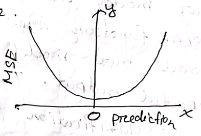
We measure how well the model fits the data using a cost function. A common cost function for linear regression is the mean squared error (MSE)
Algorithm
- Lets,
- Calculate the gradient descent
-
-
- Adjust using gradient,
-
-
- Iterate the process until converges
Example:
-
- Calculate gradients : For each iteration compute
- Learning rate,
- After multiple iteration, it finds values of that minimizes
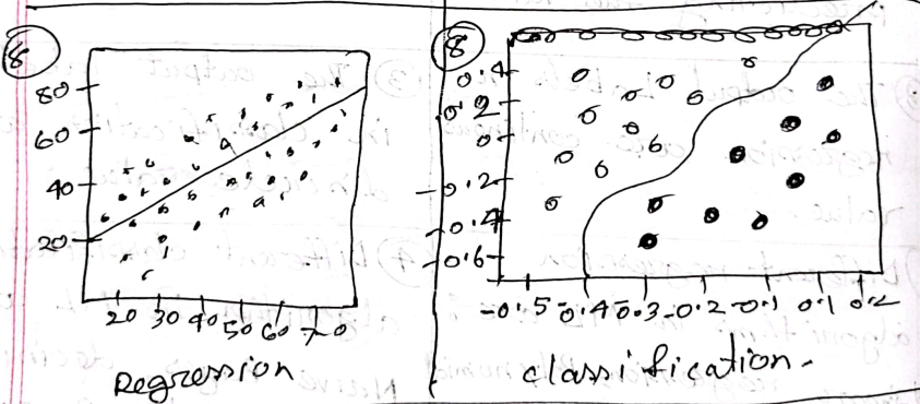
Regression and classification problems
| Aspect | Regression | Classification |
|---|---|---|
| Definition | Regression is a type of supervised learning where the algorithm learns to predict continuous values based on input feature. | Classification is a type of supervised learning where the algorithm learns to assign input to a specific category or class based on input features. |
| Used for | Predicting the values | Predicting the class |
| Output Labels | Continuous values | Discrete |
| Algorithm | Linear, Polynomial, Decision tree | Naive Bayes, Decision tree, Logistic Regression |
| Evaluation Metrics | MSE, MAE. R^2 Score | Accuracy, Precision, ROC-AUC |
| Example | Predicting house price, forecasting sales, predicting temperature, stock price | Email Classification, Disease diagnosis, image recognition, fraud detection |
Performance metrics*, AUC - ROC
https://www.tutorialspoint.com/machine_learning/machine_learning_performance_metrics.htm
Performance metrics in machine learning are used to evaluate the performance of a machine learning model.
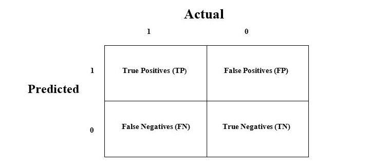
Confusion Matrix
Performance Metrics for Regression Problems
- Mean Absolute Error (MAE):
- It is basically the sum of average of the absolute difference between the predicted and actual values.
-
- Mean Square Error (MSE):
- average of the squared difference between target value and predicted value
-
- Differentiable more optimized
- Root Mean Square Error (RMSE)
- the square root of MSE
-
- Differentiable
- Handles small error done by MSE
- Score:
- R Squared metric is generally used for explanatory purpose and provides an indication of the goodness or fit a set of predicted output values to the actual output values.
-
Performance Metrics for Classification Metrics
%201.jpg)
- Accuracy
- It is the ratio correct prediction to total predictions
-
- Precision
- Proportion of true positive instances out of all predicted positive instances
-
- Defined as number of correct documents returned by our ML Model
- A precision score 1 → The model didn’t miss any true positive and is able to classify well between correct and incorrect labelling
- A low precision (<0.5) → a high number of false positive
- Recall/Sensitivity
- actual positive correctly identified
-
- Recall 1 → didn’t miss any true positive and able to classify well
- Low recall (<0.5) → high number of false negative
- Specificity
- proportion of actual negative correctly identified
-
- Score:
- Harmonic mean of precision and recall
-
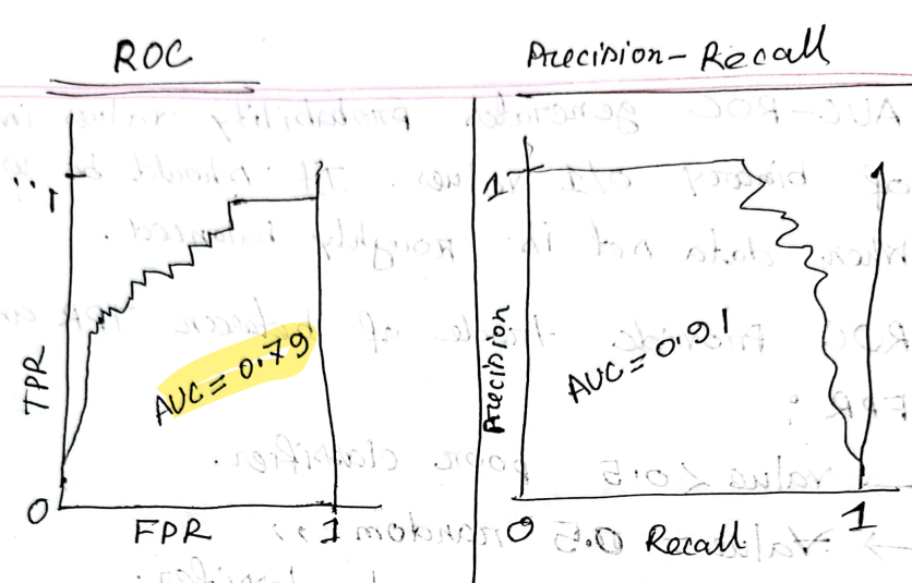
Precision-Recall Tradeoff
, can improve one a a time, but not both. So we need precision-recall combination graph to observe both.
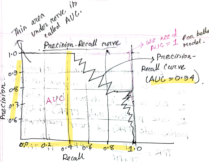
AUC
- Area Under curve
- For a better model, this should be 1
ROC AUC : Receiver Operating Characteristic Area Under Curve
https://developers.google.com/machine-learning/crash-course/classification/roc-and-auc
- ROC-AOC score is a measure of the ability of a classifier to distinguish between positive and negative instances
- The ROC curve is visual representation of model performance across all thresholds
- Calculated by TPR and FPR
- ,
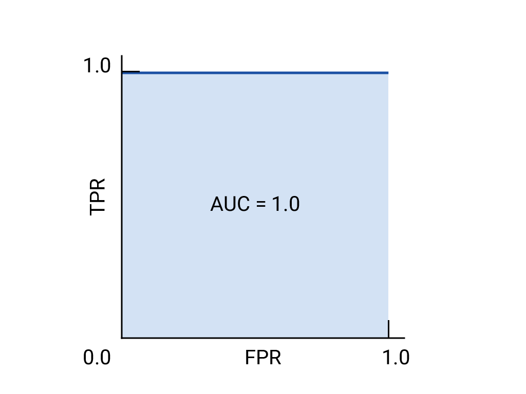
ROC and AUC of a hypothetical perfect model.
- AUC-ROC generates probability values instead of binary 0/1 values.
- It should be used where data set is roughly balanced
- ROC provides trade of between TPR And FPR
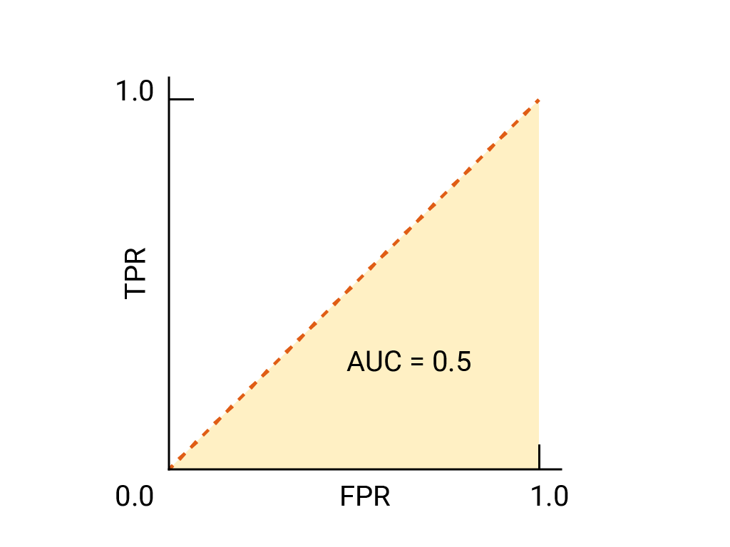
- → Poor classifier
- → Random
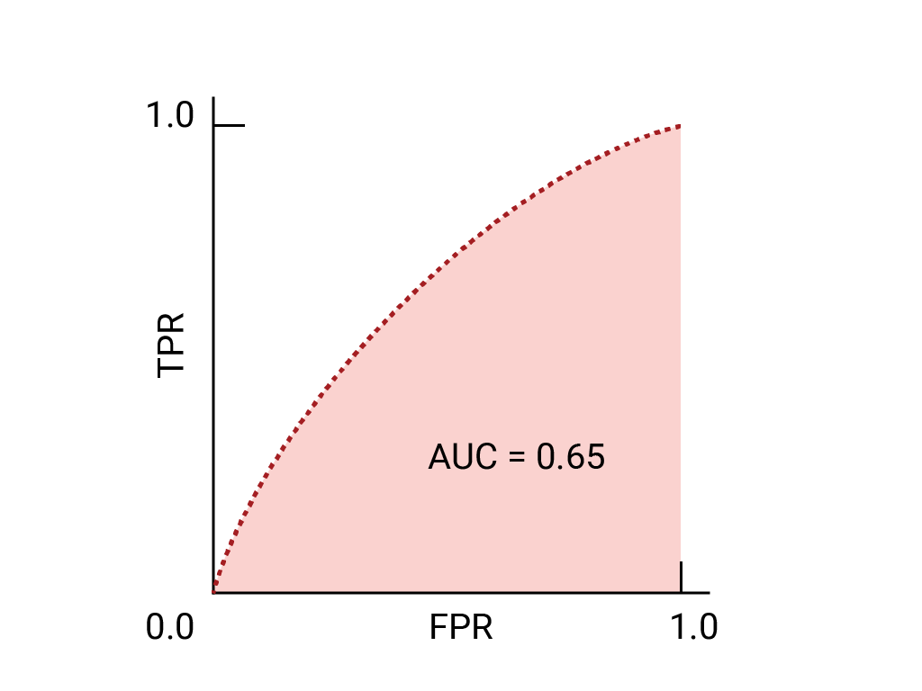
- → Good
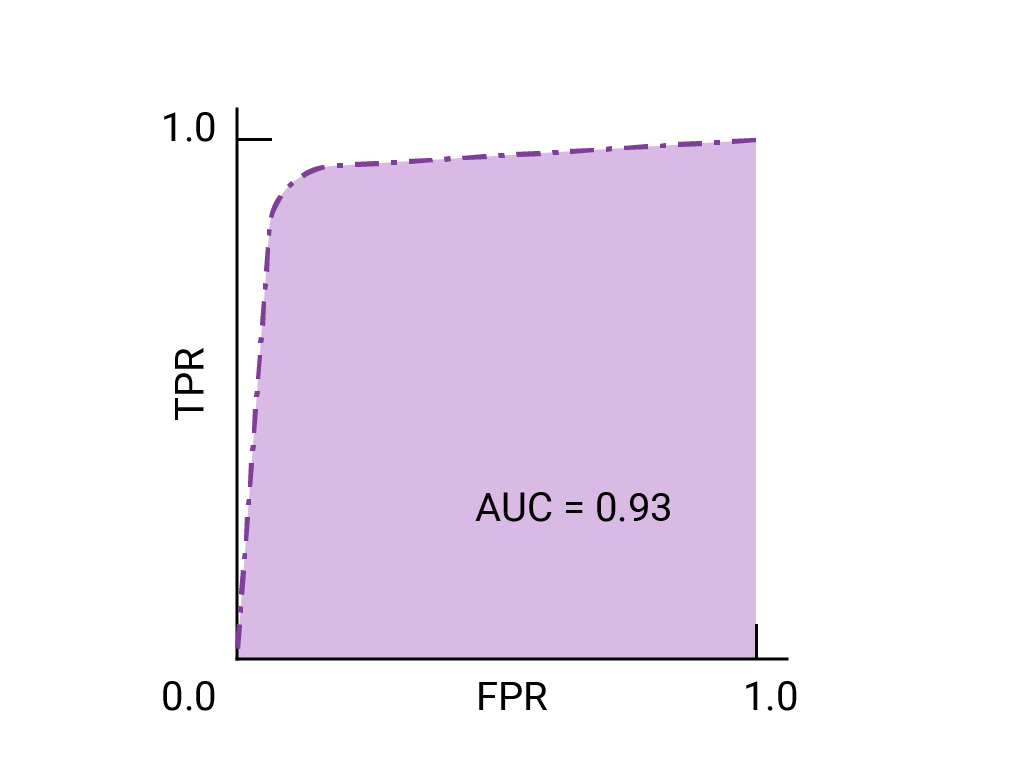
- → Indicates strong classifier
- → Perfectly predict everything
AUC-ROC Curve
Loss functions, L1, L2, Huber loss, Binary Cross Entropy loss
A loss function used in ML to measure the difference between the predicted output of a model and the actual target. Also known as cost function or error function.
Loss function for regression
- Loss
- average of absolute difference between the actual and the predicted value
-
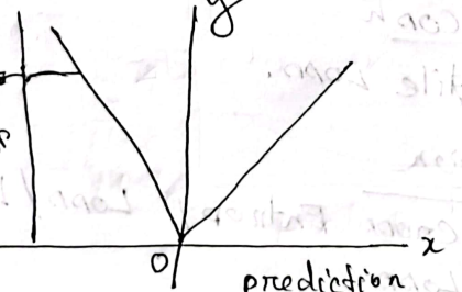
- Loss
- average of squared difference between actual and predicted value
-
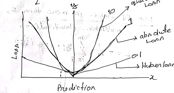
- Huber Loss
- Defined as combination of MSE and MAE loss function
- MSE → when error is small (approx. 0)
- MAE → when error is large (approx. )
- Hyperparameter controls this error to make quadratic error
-
- Defined as combination of MSE and MAE loss function
Loss functions for Classification
- Binary cross-entropy loss
- Binary cross-entropy (log loss) is a loss function used in binary classification problems
- It measures the performance of a classified model whose predicted output is a probability value between 0 to 1
- When the number of classes is 2, its binary classification.
-
- Binary cross-entropy for multiple classes ( > 2)
- Hinge Loss
- It is developed for support vector machine model evaluation
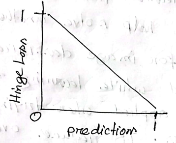
- It is developed for support vector machine model evaluation
Overfitting and underfitting in terms of bias and variance
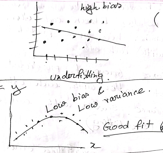
Bias : Gap between actual data of model and predicted value of data
- High Bias : Predicted value is more away than actual value (underfitting)
- Low Bias : Predicted value is near to actual value
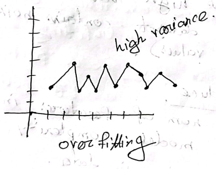
Variance: Prediction value how much scatter with relation between each other
- Low Variance : Group of predicted does not scatter
- High Variance : Scatter with each other (Overfitting)
Overfitting: Overfitting is an undesirable condition in ML that occurs when the ML gives accurate prediction for training data but not for new data.
Reasons
- High Variance and Low Bias
- Model → too complex
- Training data size → Less
- Training data → irrelevant information, noise
- Trains for too long on a single sample
Reductions
- Removing Feature
- Reduce Complexity
- Increase the size of training data
- Improve quality of training data
- Early stopping during training phase
Underfitting: It represents inability of the model to learn the training data effectively and result in poor performance both on training and testing data.
Reasons
- Too simple model
- Model has no capability to represent complexity in data
- Size of training data → less
- High Bias
- Training dataset → noise
Reductions
- Increase Complexity of model
- Increase the size of training data
- Increase number of features
- Increase duration of dataset
Activation functions, linearity and differentiability of activation functions, ReLU activation functions, use of ReLU in deep learning
Activation function is a mathematical function used in artificial neural networks to determine the output of a neuron.
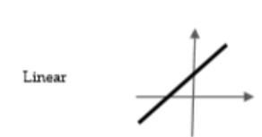
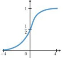
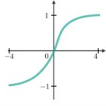
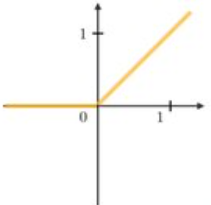
Common Activation functions
- Linear: ,
- Sigmoid:
- Tanh:
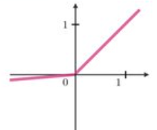
- ReLU : Reflected Linear Unit
- Leaky ReLU:
- Swish :
Activation function should be non-linear
- WHY ? To learn and represent complex and non-linear relationship between inputs and outputs
- If all activation functions are linear the NN would fail to mapping complex relation
Output Layer 1 : Output Layer 2:
If is a linear function ,
This is still a linear transformation, no matter how many layers are stacked.
- Linear activation makes deep network redundant where non-linear allows for hierarchical feature learning, complex mapping.
Activation function should be differentiable
- WHY? It can be used in process of backpropagation neural network are trained using the backpropagation algorithm which involves forward and backward passing
- backward passing requires chain rule of calculus to compute derivatives layer by layer
- So, differentiability is must
- backward passing requires chain rule of calculus to compute derivatives layer by layer
- Example: For a network output with activation function , the gradient with respect to
where and is the loss function. If f is not differentiable, the chain rule can’t propagate gradient through .
ReLU activation function
ReLU is one of the most popular activation function used in NN especially in deep learning.
It has become default choice
- simplicity and effectiveness
- positives values to pass through while setting all negative vales to zero.
- maintain necessary complex pattern
Use of ReLU
- Non-linearity
- It has constant gradient = 1 for which to mitigate vanishing gradient problem.
- Make training deep networks computationally efficient and effective
- Gradient is constant and doesn’t shrink, allowing effective backpropagate in deep learning
- Non linearity and computational simplicity
- Simple operation reduces computation
Basic structure of Artificial Neurons*
[Basic terminologies, Learning rate, momentum, threshold]
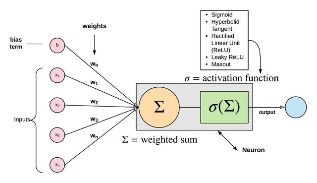
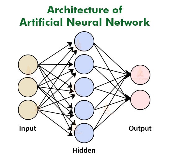
Artificial Neurons is a mathematical model to simulate how neurons process information. It is the fundamental building block of artificial neural network.
Artificial Neural Network:
- A machine learning algorithm that uses a network of interconnected nodes to process data, inspired by the human brain.
Basic components of Perceptron:
Perceptron is type of ANN (Artificial Neural Network), which is a fundamental concept in ML.
- Input Layer
- Consists of one/more input neuros
- receive signal from external world
- Weight:
- strength of the connection between input and output neuron
- Bias
- added in input layer to provide the perceptron with additional flexibility
- Activation function:
- Activation function is a mathematical function used in artificial neural networks to determine the output of a neuron.
- Output:
- a single binary value either 0/1
Basic Terminologies
- Learning Rate:
- a critical hyperparameter in ML and NN that determines the size of the steps taken during optimization process to minimize loss function.
-
- Controls how much the model updates its weight wrt the gradient
- Small LR → 0.0001 → Slow convergence
Large LR → 1.0 → Speed up Loss oscillates
LR → 0.01 → weights are update at right space.
- Momentum
- a parameter optimization technique that accelerates the gradient descent by adding a fraction of the previous update to the current update
- Reduce oscillations and improves convergence
-
- Threshold
- refers to a boundary value used to determine how a neuron behaves or how output are processed particularly in binary classification or activation function.
- Decision making
-
- A NN predicts the probability that an email is spam and the threshold is 0.5.
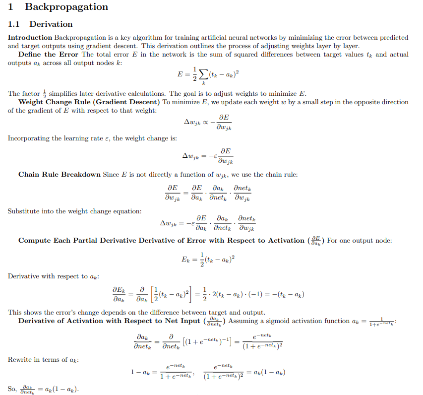
Structure of Multi-layer backpropagation network, derivation of backpropagation algorithm
Backpropagation is a fundamental algorithm for training artificial neural network. The goal of backpropagation is to reduce the difference between the models predicted output and the actual output by adjusting weights and biases.
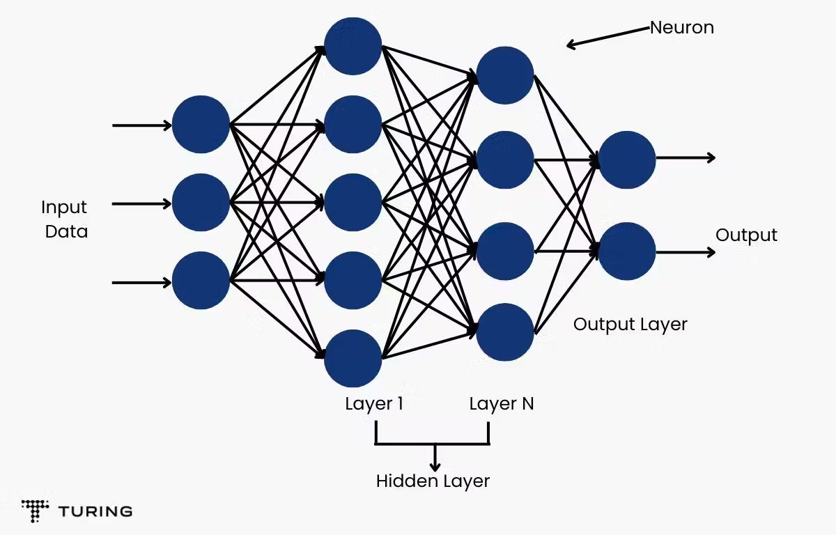
It typically consists of three main components.
- Input layer
- Hidden layer :
- intermediate layer that learn pattern from input data
- each neuron in hidden layer is connected to every in the previous and subsequent layers
- Hidden layers Network Capacity
- Output layer
- apply a suitable activation function
Derivation of backpropagation
Linearly separable and linearly non-separable problems
Convolution*, CNN*, usage of CNN*, different layers in CNN
Convolution
Convolution is a mathematical operation used in signal and image processing to extract features by applying a filter (or kernel) over an input. In the context of neural networks, this operation forms the foundation of Convolutional Neural Networks (CNNs), which are specialized for processing structured grid-like data such as images.
CNN
A Convolutional Neural Network (CNN) is a type of Deep Learning neural network architecture commonly used in Computer Vision. CNNs are particularly effective for tasks like image classification, object detection, and facial recognition due to their ability to capture spatial hierarchies and patterns. Convolutional Neural Network consists of multiple layers.
Uses of Convolutional Neural Networks
- Image classification
- Object detection
- Facial recognition
- Image segmentation
- Medical Image Analysis
- Video Analysis
Different Layers in CNN
- Input : Receives the raw input data, such as pixel values of an image, and passes it to subsequent layers for processing.
- Convolution: Applies convolution operations using filters to extract features like edges, textures, or patterns from the input data.
- Activation Layer: Introduces non-linearity (e.g., ReLU) to enable the network to learn complex patterns by transforming the convolved output.
- Pooling Layer: Reduces the spatial dimensions (e.g., max pooling) of the feature maps, retaining important information while decreasing computational load.
- Fully Connected Layer: Connects all neurons from the previous layer to produce high-level reasoning, consolidating features for final decision-making.
- Output Layer: Generates the final output, such as class probabilities or a classification label, based on the processed features
RNN, uses of RNN, vanishing and exploding gradients problems, how solved?* Architectural difference between LSTM and GRU*
Recurrent Neural Networks (RNNs) are a class of neural networks designed to handle sequential data by maintaining a memory of previous inputs through recurrent connections.
Uses of Recurrent Neural Networks
- Natural Language Processing
- Time series prediction
- Speech recognition
- Machine translation
Vanishing and Exploding Gradients Problems
During backpropagation through time (BPTT) in RNNs, the following issues arise:
- Vanishing Gradients: Gradients become extremely small as they are propagated back through many time steps, causing early layers to learn slowly or not at all.
- Exploding Gradients: Gradients grow excessively large, leading to unstable training and large weight updates that disrupt learning.
Solutions to Vanishing and Exploding Gradients
- Gradient Clipping: Limits the gradient magnitude during backpropagation to prevent exploding gradients by capping values above a threshold.
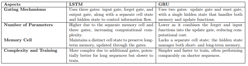
- Long Short-Term Memory (LSTM) Units: Introduces memory cells and gates (input, forget, output) to preserve long-term dependencies, mitigating vanishing gradients
- Gated Recurrent Units (GRU): A simplified version of LSTM with update and reset gates, improving gradient flow and reducing vanishing gradient effects.
- ReLU Activation: Replaces traditional activations to avoid the saturation issues that contribute to vanishing gradients
Architectural Differences Between LSTM and GRU
Long Short-Term Memory (LSTM) and Gated Recurrent Units (GRU) are advanced recurrent neural network architectures designed to mitigate the vanishing gradient problem. This document compares their architectural differences in a tabular format.
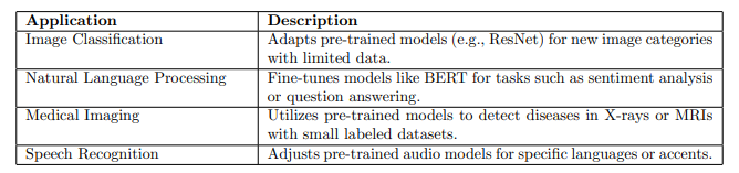
Transfer learning*, usage*
Transfer learning is a machine learning technique where a model trained on a large, general dataset is fine-tuned for a specific task with a smaller dataset.
Transfer learning is a machine learning technique where knowledge gained from solving one task is leveraged to improve a model’s performance on a different but related task. Instead of training a model from scratch for every new problem, transfer learning uses a pre-trained model—typically trained on a large dataset for a source task—and adapts it (often by fine-tuning) for a target task, which may have less data or slightly different requirements
Usage
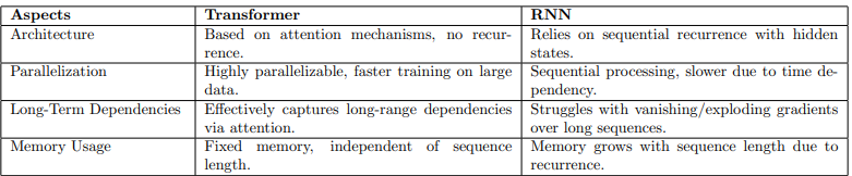
Transformer model*, Attention mechanism in transformer architecture*, Transformer vs RNN*.
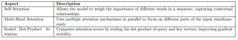
The Transformer model is a deep learning architecture introduced for sequence-to-sequence tasks, relying entirely on attention mechanisms and eliminating recurrent structures.
A transformer model is a type of neural network architecture that has revolutionized the field of artificial intelligence, especially in natural language processing (NLP) and other sequential data tasks. Introduced in the 2017 paper ”Attention is All You Need,” transformers have become the foundation for many modern AI systems, including large language models and generative AI.
Attention mechanism
Transformer vs RNN